VEGA
Molecular Modeling Toolkit
Printable manual
1. Introduction
VEGA was developed to create a bridge between most of the molecular software packages, as Quanta/CHARMm, Insight II, Mopac, etc. In this tool, some features have been implemented to analyze and manage 3D structures of molecules. VEGA is written in high portable code (standard C language) and can be executed on a lot of hardware systems simply recompiling the source code. The program is already tested on the following operating systems: IRIX (Silicon Graphics), Windows 9x/NT/2000/XP/Vista/7/8 PCs, Linux, FreeBSD, NetBSD, AmigaOS, etc.
The most significant features implemented in VEGA are:
Supported input file formats: Alchemy, AMMP, Accelrys Insight .car and .arc, Accelrys Quanta/CHARMm CRD, AutoDock 4 PDBQT, AutoDock Vina PDBQT, CSR, MSF and DCD, CML 1.0 and 2.0, BioDock output, Cambridge Data File (CSSR), Chem3D, ChemDraw CDX, ChemSol, Cartesian coordinates (XYZ), CPMD XYZ, EMPIRE .arc and .dat, ESCHER NG solutions, GAMESS cartesian input and output, Gaussian cartesian input and output, GRAMM solutions, Gromos/Gromacs .gro and .xtc, HyperChem .hin, InChI, Interchange File Format (IFF/RIFF), IUCr Crystallographic Information Framework (CIF, mmCIF), IUMSC CRT, LiGen binary/text pocket, MDL Molfile, Mopac cartesian coordinates, Mopac internal coordinates, Mopac Guassian Z-matrix, NAMD binary, Protein Data Bank (PDB), Data Bank with ATDL atom types (PDBA), Protein Data Bank Fat (PDBF), PQR, PQR XML, Protein Data Bank MultiModel, QMC, SMILES, Spillo RBS, TINKER XYZ, Tripos Sybyl (Mol2), X-Plor PSF.
Supported output file formats: Accelrys Insight .car (archive 1 and 3), Accelrys Quanta/CHARMm CRD and MSF, Alchemy, AMMP, AutoDock 4 PDBQT, AutoDock Vina PDBQT, Cambridge Data File (CSSR), Cartesian coordinates (XYZ), ChemSol, CML 1.0 and 2.0, CPMD XYZ, Crystallographic Information Framework for macromolecules (mmCIF), Fasta, GAMESS cartesian, Gaussian cartesian input, Gromos/Gromacs .gro, InChI, InChI Aux, Interchange File Format (IFF), IUCr Crystallographic Information Framework (CIF), IUMSC CRT, MDL Molfile, Mopac cartesian coordinates, Mopac internal coordinates, NAMD binary, Protein Data Bank (PDB), Protein Data Bank with ATDL atom types (PDBA), Protein Data Bank with atomic charges (PDBQ), Protein Data Bank Fat (PDBF), Protein Data Bank with more than 99999 atoms (PDBL), Protein Data Bank simplified, PQR, PQR XML, SMILES, Spillo RBS, Tripos Sybyl (Mol2), VRML.
Supported output surface formats: CSV, IFF/RIFF, Insight, Quanta, raw binary, VRML.
Supported output trajectory formats: Charmm DCD, IFF/RIFF, Mol2 multi-model, PDB multi-model, Gromacs TRR and Gromacs XTC.
Atomic charge attribution by Gasteiger method or a template of residues.
Atom type attribution. The supported atom types are: AM1BCC, AMBER, AutoDock, Bond, Broto/Moreau (BROTO), CFF91, CHARMm, CHARMM 22 for nucleic acids (CHARMM22_NA), CHARMM 22 for lipids (CHARMM22_LIPID), CHARMM 22 for proteins (CHARMM22_PROT), CHARMM 36 (CHARMM36_GEN), CVFF, Ghose/Crippen (CRIPPEN), Ghose/Crippen for molar refractivity (CRIPPEN_MR), functional groups (GROUPS), GRID, H-bond (HBOND), logS, Meng, MM+, MM2, MM3, MMFF, Tripos, UNIV and any other user defined template. A simple language to define the atom types is built-in (ATDL).
Calculation of molecular surfaces (Van der Waals, accessible to solvent, Molecular Electrostatic Potential (MEP), Molecular Hydropathicity Index (ILM) and Virtual logP (MLP)).
Capability to add the hydrogens.
Calculation of ligand-receptor interaction energy for each residue involved in the binding.
Evaluation of logP (Broto/Moreau, Ghose/Crippen, Virtual logP) and lipole (Broto/Moreau, Ghose/Crippen).
Evaluation of the molecular refractivity (Ghose/Crippen method).
Analysis of MD trajectories. VEGA can read: Accelrys archive file (.arc), AutoDock 4 DLG, BioDock output, CSR (Accelrys conformational search), DCD, ESCHER NG, GRAMM, Gromacs TRR, Gromos XTC, IFF/RIFF (32 and 64 bit), Crystallographic Information Framework multi-model (CIF, mmCIF), MDL Mol multi-model, Merck MMD, Tripos Mol2 multi-model, PDB multi-model and PDBQT multi-model file formats. It's possible to calculate several properties as the interatomic distance, the bond angle, the torsion, the angle between two planes, the molecular surface, the surface diameter, the molecular volume, the volume diameter, the dipole, the Virtual logP.
Molecule extraction from databases (IUPAC names, Microsoft Access, Merck MMD, Mol2, ODBC, SMILES, Sdf, SQLite and Zip).
Coordinates normalization.
Molecule solvation with any type of cluster.
Deletion of water molecules and hydrogen atoms.
Residue renumbering.
OpenCL acceleration for both Windows and Linux versions.
2. Installation
The VEGA package is available in different archives/setups:
| Vega_ZZ_X.X.X.X_Setup.exe |
Windows x86/x64 (32/64 bit) setup wizard with OpenGL and OpenCL support. This is the main package that must be installed first. Now it includes the LiveCD Creator utility that is not more available as separated setup. |
| Vega_ZZ_X.X.X.X_MassTools.exe | Mass spectrometry plug-in. For more information, click here. |
Vega_X.X.X_Irix6.2.tar.gz |
SGI IRIX 6.x command-line version. |
Vega_X.X.X.X_Linux_x86-x64-ARM.tar.gz |
Linux x86 (32 bit), x64 (64 bit) and ARM (VFP) command-line versions. The OpenCL support is available only for x86 and x64 versions. |
Vega_X.X.X_Amiga.lha |
AmigaOS 68k command-line version. |
| Vega_X.X.X.X_Locale.tar.gz | Localization toolkit. |
where X.X.X and X.X.X.X are the release version of each archive/setup. You you can download only the package for your system, because each archive contains all the files needed, but not the source code that is provided in a separate archive.
2.1 Unix installation
This section of the manual shows the steps needed to install the VEGA package on Unix-like operating systems (e.g. IRIX, Linux, NetBSD, etc). If your operating system is not directly supported by Authors, you must download and compile the source code (Vega_X.X.X_Source.tar.gz archive).
2.1.1 Building the VEGA package
The portable source code allows to build the package virtually for any computer platform that has a standard ANSI C compiler. It is possible to find some minor compiling problems due to hardware differences. If you can't solve these problems, please contact the Authors.
As first step, you must unpack the Vega_XX_Source.tar.gz file, using the gzip command. If this command is not available in your system, you can download it from any GNU software archive (see: http://www.opensource.org). The correct syntax is:
gzip -d Vega_X.X.X_Source.tar.gz
the unpacked file (Vega_X.X.X_Source.tar) created by gzip must be dearchived with tar command:
tar -xvf Vega_X.X.X_Source.tar
A directory called Vega will be created.
Check if the libraries libbz2.a, loblocale.a, libxdrf.a, libz.a and libZ32.a are present in the directory ...Vega/Src/Vega/MySO where MySO is the directory of your operating system. If not, you must compile these external libraries using the sources placed respectively in ...Vega/Src/Bzip2, ...Vega/Src/LocaleLib, ...Vega/Src/XdrfLib, ...Vega/Src/Zlib and ...Vega/Src/Z32 editing the Makefile and running make. Each library must be copied in ...Vega/Src/Vega/MySO.
After this operation, change your current directory in ...Vega/Src/Vega/MySO (Amiga, Irix, Linux, Unix, Win32) and, if needed, edit the Makefile with your preferred program. Some remarks can help you in this operation. Please set the CC variable to the compiler name (usually cc or gcc) and the CFLAGS variable for the best optimization (e.g. -O -s).
At this point, run make and the VEGA executable is compiled for your system. The makefile was successfully tested with SGI cc and GNU C (gcc for Linux, gcc for AmigaDOS) compilers.
WARNING:
Starting from the 1.5.0 release, it was introduced the use of 64 bit integers to
speed-up the manipulation of 8 character strings and thus to build VEGA, it's
required a C compiler that supports that integer size.
2.1.2 Setting-up your Unix system
If the downloaded package has been specifically developed for your operating system, you must unpack it using the following two commands:
gzip -d Vega_X.X.X_MyOS.tar.gz
tar -xvf Vega_X.X.X_MyOS.tar
If you have GNU tar, you can even do it in one step only:
tar -zxvf Vega_X.X.X_MyOS.tar.gz
Please note that the pathway where the archive has been unpacked, is the real installation path.
Test installation
Type the command (one time only):
chmod -R 755 Vega/Bin/*
and every time that you need VEGA:
cd Vega
source ./assign.sh
In this way, the more suitable set of binaries is automatically detected and its folder is added to the command search path.
Full installation
The next step is the editing of your shell start-up script (e.g. .cshrc for csh or
tcsh, .bashrc for GNU bash) in order to set VEGADIR
and the LD_LIBRARY_PATH environment variables
to the installation path. For csh/tcsh shell, you must type:
setenv VEGADIR "<INSTALLATION_PATH>"
setenv LD_LIBRARY_PATH "$VEGADIR/Bin/<MyOS> $LD_LIBRARY_PATH"
setenv PATH "$VEGADIR:$PATH"
where <MyOS> is the operating system (e.g. Linux_x64, Linux_x86, etc) and <INSTALLATION_PATH> is the full installation path.
For sh/bash:
export VEGADIR="<INSTALLATION_PATH>"
export LD_LIBRARY_PATH="$VEGADIR $LD_LIBRARY_PATH"
export PATH="$VEGADIR/Bin/<MyOS>:$PATH"
The LD_LIBRARY_PATH is required to inform your system where are the dynamic libraries needed by VEGA. It's strongly recommended to add the installation directory pathway in the command search variable path, defined in shell start-up script.
For example, if you installed VEGA for Linux x64 in /usr/local/vega
directory, you must set the environment variables (csh/tcsh):
setenv VEGADIR "/usr/local/vega"
setenv LD_LIBRARY_PATH "$VEGADIR $LD_LIBRARY_PATH"
setenv PATH "$VEGADIR/Bin/Linux_x64:$PATH"
or (sh/bash):
export VEGADIR="/usr/local/vega"
export LD_LIBRARY_PATH="$VEGADIR $LD_LIBRARY_PATH"
export PATH="$VEGADIR/Bin/Linux_x64:$PATH"
Finally, you must change the file permissions:
chmod -R 755 $VEGADIR/Bin
To set the localization language of VEGA program, you can edit the <INSTALLATION_PATH>/Config/prefs file: find the <LANGUAGE> item and select your preferred language (at this time, two languages are supported only: english and italian). The automatic language selection isn't supported by Unix operating systems. The installation can be completed enabling the OpenCL acceleration, if the host operating system is Linux x86/x64.
2.1.2 Linux and OpenCL
If your system is equipped with an OpenCL-enabled device (a GPU or an accelerator) and its driver is correctly installed, VEGA recognizes and uses it automatically. For AMD GPUs (HD4000 series and above) and for systems not equipped with a OpenCL-ready GPU, you must install the ATI Stream SDK. In the second case, the OpenCL acceleration is available even if a compatible GPU is not installed, by the CPU that must support SSE2 instruction set to emulate the OpenCL environment. Although the performance aren't comparable to a real OpenCL device, you can obtain a speed-up due to the massive use of the SIMD instructions by the real-time OpenCL compiler.
To install the ATI Stream SDK:
tar -xvzf ati-stream-sdk-vX.X-lnxYY.tgzwhere X.X is the SDK version and YY could be 32 or 64 on the basis of the version chosen by you. Remember that the examples and the C includes aren't required by VEGA and if you don't want to develop OpenCL application, you can remove the docs, include, make and samples directories to shrink the installation.
export ATISTREAMSDKROOT=<location where the SDK is installed>
export ATISTREAMSDKSAMPLESROOT=$ATISTREAMSDKROOT # Required if you want build the examples
For 32-bit systems:
export LD_LIBRARY_PATH=$ATISTREAMSDKROOT/lib/x86:$LD_LIBRARY_PATHFor 64-bit systems:
export LD_LIBRARY_PATH=$ATISTREAMSDKROOT/lib/x86_64:$LD_LIBRARY_PATH
cd /
tar -xvzf icd-registration.tgz
If you have a Nvidia OpenCL enabled graphic card (GeForce 8 series and above with at least 256 Mb of ram), download and install the latest CUDA Toolkit for Linux.
If you find any problem using the OpenCL acceleration, see the prefs file in the Data directory to enable/disable or to select devices.
2.2 Windows installation
This release contains two versions: the console (command
line) and the ZZ (OpenGL) versions. The first one is a true Win32 console application. It supports long
filenames and works fine with Windows 2000, XP, Server 2003,
Vista, Server 2008 and 7 operating
systems (x86 and x64 editions). The package has been compiled using the standard Pentium
Pro ® (686) instruction
set. The
second version is a powerful application with an enhanced graphic interface. For
more information, go to VEGA ZZ section.
To install the Vega_ZZ_XX_Setup.exe package, you must execute this file
and follow the simple installation wizard. You must remember that you must have
the administrator rights to complete the installation.
If your system has a software firewall, you must configure it granting the
network access to REBOL.exe, otherwise the scripting system doesn't work because
it uses the standard TCP/IP communication ports.
After the installation, run VEGA ZZ and the activation procedure starts.
The setup can be completed installing the
optional components and enabling the OpenCL
acceleration.
2.2.1 Windows and OpenCL
As explained in the Unix/Linux installation section, if your system is equipped with an OpenCL-enabled device (a GPU or an accelerator) and its driver is correctly installed, VEGA and VEGA ZZ recognize and use it automatically. For AMD GPUs (HD4000 series and above) the OpenCL driver is included in the standard driver package. For the systems not equipped with a OpenCL-ready GPU, you can install ATI Stream SDK which provides the OpenCL acceleration emulated by the CPU that must support SSE2 instruction set. Although the performance aren't comparable to a real OpenCL device, you can obtain a speed-up due to the massive use of the SIMD instructions by the real-time OpenCL compiler.
To install the ATI Stream SDK:
If you have a Nvidia OpenCL enabled graphic card (GeForce 8 series and above with at least 256 Mb of ram), download and install the latest CUDA Toolkit for Windows.
If you find any problem using the OpenCL acceleration, see the Preferences window to enable/disable or to select devices.
2.3 AmigaDOS installation
System requirements needed to run the AmigaDOS version of VEGA:
To install this version of VEGA package, you must unpack the distribution archive using lha command from the command shell:
lha x Vega_XX_Amiga.lha
A directory called Vega will be automatically created. If you don't have lha, you can download it from Aminet. As for Unix systems, you must add in the user-startup file (placed in s directory of your boot disk) the following line:
SetEnv VEGADIR <INSTALLATION_PATH>
Instead of the user-startup modification, you can create a new text file in ENVARC: directory containing a single line with the installation pathway. Starting from 1.2 release, this installation step is needed only if VEGA executable is placed in a directory that is not the installation folder.
If you want to add VEGA to your standard command pathway, you can add in the user-startup the following line:
Path <INSTALLATION_PATH> Add
As final step, reboot your computer. Please note that VEGA for Amiga can accept AmigaDOS and Unix-like pathway specification. Use the specific VEGA version for the CPU installed in your system:
| Version | CPU |
| VEGA.000 | 68000, 68010 and any other CPU without FPU. |
| VEGA.020 | 68020 and 68030 with 68881/2 FPU. |
| VEGA.040 | 68040 and 68060. |
The PowerPC CPUs aren't supported.
3. Usage
Running the program without parameters, the list of the implemented options is shown:
VEGA 3.2.3 - (c) 1996-2023,
Alessandro Pedretti & Giulio Vistoli
Virtual logP by Bernard Testa et al.
Windows x64 (64 bit) version
Synopsis: vega INPUT ...
-o[OUT.PACK] -f[OUTPUT_FORMAT]
-p[FORCE_FIELD]
-s[POINTS] -g[RADIUS]
-c[TEMPLATE] -k[KEYWORDS]
-a[RES_NUM]
-d[DIELECTRIC] -e[MOLNUM]
-i[SHELL RAD SHAPE]-j[TORSIONS]
-l[MOLTYPE]
-m[KEYWORDS]
-q[METHOD]
-r[MODE]
-t[SECSTRUCT]
-v[CPUS] -x[MODE
(ID)]
-z[NTERM CTERM]
-0bhnuwy
0 -> ignore locale
settings of the decimal separator
a -> renumber residues starting from RES_NUM
b -> don't save the connectivity
c -> charge template (FORMAL, GASTEIGER,
...)
d -> dielectric constant for energy calculation
e -> molecule number for score calculation (0
= last)
f -> output format
g -> probe radius for SAS
h -> show this help
i -> solvate the molecule
j -> define the torsions (ALL, AUTODOCK, FLEX)
k -> keywords for InfoXML and MopInt
l -> add hydrogens (GEN, GENBO, NA, NABO, PROT, PROTBO)
m -> keywords for trajectory analysis
n -> normalize coordinates
o -> output file name
p -> define force field to apply
q -> fix the bond order (ALL, RINGS)
r -> remove hydrogens (ALL, APOLAR)
s -> point density for SAS
t -> change the protein secondary structure
u -> add the side chains to a protein
v -> number of CPUs (0 = all)
w -> remove waters
x -> list/extract molecule/s from a database (LIST; NAME name; NUM number)
y -> find the molecules in the assembly
z -> N-term and C-term capping for peptide (default: NONE
NONE)
INPUT formats:
Alchemy, AMMP, Arc, AutoDock 4 DLG, BioDock, CAR, CHARMM CRD, CIF, CML,
CML 2.0, CPMD XYZ, CRT, CHARMM DCD, Chem3D, ChemDraw CDX, ChemSol, CSSR,
EMPIRE, ESCHER NG, Fasta, GAMESS, Gaussian In/Out, GRAMM, Gromacs/Gromos
mol, Gromacs TRR, Gromacs XTC, HIN, IFF, InChI, LiGen pocket, MDL,
MDL V3000, Mol2, Mopac cartesian, Mopac Gaussian Z-matrix, Mopac internal,
MSF, NAMD binary, PDB, PDBA, PDBF, PDBL, PDBQT, PQR, PQRXML, PSFX, QMC,
Quanta CSR, RIFF, SDF, TINKER XYZ, XYZ, ZIP.
OUTput formats:
Calc: Info, InfoXML,
Score.
Map: BiosymSrf, ComfaFld, CsvIlm, CsvLogP, CsvMep, CsvSrf,
QuantaIlm, QuantaLogP, QuantaMep,
QuantaSrf.
Molecule: Alchemy, AMMP, Biosym, ChemSol, CIF, CML, CML2, CPMDXYZ, CRD,
CRT, CSSR, Fasta, GAMESS, GaussIn, Gromos, GromosNm, IFF,
InChI, InChIAux, InChIKey,
Indigo, MdlMol, MdlMol3, mmCIF,
Mol2, MopCar, MopInt, MSF, NamdBin, OldBiosym, PDB, PDB2,
PDBQ, PDBA, PDBF, PDBL, PDBNOTSTD, PDBQT, PQR, PQRXML,
PSFX, QMC,
RIFF, SMILES, SpilloRBS, VINA, XYZ.
Plot: BinPlt, CSV, QuantaPlt.
Trajectory: TrjDCD, TrjIFF, TrjMol2, TrjPDB, TrjTrr,
TrjXtc.
VRML: Vrml, VrmlPts, VrmlCpk,
VrmlSol.
PACKer formats:
bz2 (BZip2), gz (GZip), pp (PowerPacker), z (Z-Compress).
Score functions (-f Score -k):
Broto, Broto2, Broto3, Charmm, Charmm22, Charmm36, CVFF, Elect, ElectDD.
TRAJECTORY keywords (-m):
Angle A1 A2 A3, Dipole, Distance A1 A2, Extract F1 [F2], GyrRad, ILM,
LipoleBr, LipoleCr, Ovality, PlaneAng A1 A2 A3 A4 A5 A6, PSA, RMSD,
RMSDH, RMSDALN, RMSDALNH, RMSDSYMCOR, RMSDSYMCORH, Surface A1 ...,
SurfDia A1 ..., Torsion A1 A2 A3 A4, VlogP, VolDia, Volume.
Secondary structure keywords (-t):
AlphaHelix, LeftHelix, 310Helix, PiHelix, Beta, BetaAnti, BetaPar.
or
TOR=VALUE TOR=VALUE ...
where TOR is the torsion name (Phi, Psi, Omega) and VALUE is the
torsion value in degree.
Peptide capping keywords
(-z):
NTERM: NONE, H3N+, HCONH, H3CCONH
CTERM: NONE, O-, OH, OCH3, OC2H5
All parameters are optional with the exception of the input file name (INPUT).
3.1 INPUT ...
This option allows to specify the input file names. VEGA recognizes
automatically the format of input files and the list of supported input
formats is shown running VEGA without arguments.
You can load more than one file at once with the same or different file formats to create
molecular assemblies. The calculation of connectivity is performed separately for each
file to prevent connectivity errors when the molecules are overlapped.
The Data Decompressor Engine allows to manage compressed files as
normal unpacked files without any
external data decompressor. VEGA supports the following compression formats:
| Format name | File extension |
| BZip2 | .bz2 |
| GZip | .gz |
| PowerPacker | .pp |
| Unix Un/compress | .Z |
VEGA can recognize .url files and open URLs specified as file names, downloading the molecules for you.
3.2 -0
With this option, VEGA ignores the locale settings and writes always a dot (.) as decimal separator.
3.3 -a[RESNUM]
This option renumbers all residues starting from [RES_NUM]. If this value is not specified, VEGA starts from one. The residue renumbering is very useful when you create an assembly starting from two or more molecules.
3.4 -b
This switch saves molecules without connectivity records when the output format can store this kind of information (e.g. PDB, PDBF, IFF). Many molecular packages interpret incorrectly the CONECT field in PDB files, therefore, to solve this problem, you can save the molecule without connectivity.
3.5 -c[TEMPLATE]
Currently, VEGA supports formal charges (formal keyword), atomic charges based on a fragment database (charmm22_char, charmm36_char, opls_char keywords) and atomic charges based on the Gasteiger-Marsili method (gasteiger keyword) . The Gasteiger-Marsili approach is based on a multi-step procedure:
The formal charges are correctly assigned only if all bonds have the right order (single, double and triple).
3.6 -d[DIELECTRIC]
Use this option If you want to calculate the interaction energy (see -f[FORMAT] option) changing the default dielectric constant (1.0). Please note that the default value of dielectric constant is stored in the prefs file.
3.7 -e[MOLNUM]
This is a compulsory parameter for the interaction energy evaluation (docking score evaluation, see -f[FORMAT] option). It is required to know which molecule (ligand) is considered to evaluate the interaction energy. You can specify 0 as molecule number to indicate the last molecule in the assembly.
WARNING:
the IFF/RIFF file format is the only one that is able to contain the molecule
number information. For this reason, it's impossible to select the ligand by
molecule number if you use assemblies (files containing more than one molecule)
in other formats. To skip the problem, you can build the assembly on-the-fly
specifying the ligand and the receptor as in the following example:
vega receptor.pdb ligand.pdb -f score -c gasteiger -k "CHARMM36 ELECT" -e 0 -o receptor-ligand.xml
Another solution is the use of -y options that enables the detection of molecules:
vega assembly.pdb -f score -c gasteiger -k BRORO -e 2 -o score.xml -y
3.8 -f[OUT.PACK]
With this parameter, you can create an output file in a specific file format. If -f is omitted, the default output format is PDB full standard (see PDB specifications) unpacked. OUT indicates the format and PACK is the optional compression method (bz2, gz, pp and z, see INPUT). This two keywords are case-insensitive.
| e.g. | -f CSSR | CSSR output without compression. | ||
| -f pdb.Z | PDB output with Unix compression. | |||
| -f xyz.bz2 | XYZ output with BZip2 compression. |
3.8.1 Calculation formats
| Keyword | Description |
INFO |
Information about the molecule. |
| INFOXML | Same of above but the results are included in a XML file. |
| Score | Evaluation of interaction energy (molecular docking score). |
3.8.1.1 Information about the molecule
If you want more information about the input molecule, you can use -f INFO option. When you select this operation, VEGA shows many information: total number of atoms, number of heavy atoms, number of residues, number of molecules contained, number of water molecules, molecular weight, coordinates of geometric center, coordinates of mass center, approximative dimensions, total charge (calculated using the atomic charges), dipole, surface area, surface diameter, volume, volume diameter, ovality (only if the probe radius used for surface calculation is null, see -g option), Crippen's logP and lipole, Broto's logP and lipole, Virtual logP (available only in full release), predicted charge (only for proteins, it's calculated searching ionizable groups), aminoacidic charge (only for proteins, it's calculated at physiological pH on the basis of aminoacidic composition), aminoacidic or nucleotidic composition:
************************************
**** Information about molecule ****
************************************

Atoms..............: 48
Heavy atoms........: 25
Residues...........: 1
Molecules..........: 1
Waters.............: 0
Formula............: C19H23NO5
Molecular weight...: 345.384 Daltons
Monoisotopic mass..: 345.157623 Daltons
Geometry center....: 7.1076 3.6789 0.5790
Mass center........: 6.9492 3.5914 0.5256
Appx. dimensions...: 17.4088 10.7721 10.7163
Total charge.......: 0.0003
Dipole.............: 1.0292 Debye
Surf. area (0.00)..: 383.3 Ų (ds=11.0 Å)
Polar area (PSA)...: 50.6 Ų (apolar=332.7 Ų)
Volume.............: 362.3 ų (dv=8.8 Å)
Ovality............: 1.6
logP (Crippen).....: 1.9275
Lipole (Crippen)...: 0.4363
logP (Broto).......: 3.0390
Lipole (Broto).....: 0.4755
Virtual logP.......: 3.1402
Please note that the total number of atoms exceeds the MAXATMINFO key in prefs file, surface area, surface
diameter, volume, volume diameter, ovality and logP values are not shown.
If the molecule is a protein or a nucleic acid, the following data are shown:
...
Total charge.......: -23.0004
Predicted charge...: -24
Aminoacidic charge.: -24
Aminoacidic composition:
Res    N.   N. %     Mass     Mass %
====================================
ALA    46   6.29  3269.690    3.57
ARG    42   5.75  6618.506    7.22
ASN    29   3.97  3309.140    3.61
ASP    43   5.88  4921.520    5.37
CYS    18   2.46  1855.515    2.02
GLU    53   7.25  6789.680    7.41
GLN    46   6.29  5894.132    6.43
GLY    40   5.47  2282.165    2.49
HIS    26   3.56  3565.805    3.89
ILE    37   5.06  4186.861    4.57
LEU    86  11.76  9731.422   10.62
LYS    30   4.10  3875.539    4.23
MET    11   1.50  1443.115    1.57
PHE    25   3.42  3681.328    4.02
PRO    35   4.79  3401.088    3.71
SER    42   5.75  3657.370    3.99
THR    24   3.28  2426.550    2.65
TRP    17   2.33  3165.578    3.45
TYR    35   4.79  5710.992    6.23
VAL    46   6.29  4560.075    4.98
WARNING:
If the protein doesn't have got hydrogens, the predicted charge isn't shown. If
protein contains special non-aminoacidic groups and/or metal ions, the predicted
charge can be incorrect.
3.8.1.2 Evaluation of interaction energy (molecular docking score)
VEGA can evaluate the ligand-biomacromolecule interaction energy through molecular mechanics calculations. Some scoring functions are implemented (for more details, see -k option).At the present time, only the CVFF force field is implemented. Please remember that ligand and receptor must have correctly assigned charges (see -c option) if you want to calculate the electrostatic interaction. You can specify the dielectric constant with -d option (default 1.0) and the ligand (see -e option). After the energy calculation, VEGA shows (or writes in a XML file) the total interaction energy, the components for each atom and residue.
3.8.2 Molecule formats
| Keyword | Description |
| ALCHEMY | Alchemy format. |
| AMMP | AMMP molecular mechanics software. |
BIOSYM |
New Biosym .car file (archive 3). |
| ChemSol | ChemSol 2 solvatation energy software. |
| CIF | IUCr Crystallographic Information Framework. |
| CML | Chemical Markup Language (CML) version 1.0. |
| CML2 | Chemical Markup Language (CML) version 2.0. |
CRD |
CHARMM text file format. |
| CRT |
Indiana University Molecular Structure Center (IUMSC) CRT format for crystallographic structures. |
| CPMDXYZ | CPMD (Car-Parrinello Molecular Dynamics Code) Cartesian output file. |
CSSR |
Cambridge Data File. |
FASTA |
FASTA is not a real molecular file, because it can store only the primary structure of proteins and DNA/RNA sequences. |
| GAMESS | Cartesian GAMESS format. |
| GAUSSIN | Gaussian Cartesian input. |
GROMOS |
This is the special file format of the molecular mechanics package Gromos/Gromacs. |
GROMOSNM |
GROMOS with the coordinates in nanometers. |
IFF |
Interchange File Format. This is a binary file with an AmigaOS chunk structure (like IFF-ILBM, AIFF, etc). All chunks are optional and the structure is totally expandable (see Appendix D). |
| INCHI | IUPAC Chemical Identifier (InChI). |
| INCHIAUX | Same of above with auxiliary data. |
| INFOXML |
This is not a real file molecule file format, because it's a XML container of property data only. The user can select the properties to calculate including the -k[KEYWORDS] option. |
| MDLMOL | MDL Molfile. |
| MMCIF | Crystallographic Information Framework for macromolecules. |
MOL2 |
Tripos Sybyl Mol2 file format. |
| MOPCAR | Mopac cartesian coordinate file (see below). |
MOPINT |
The Mopac internal coordinates file (.dat) is useful to link Mopac with other software packages. The Mopac keyword CHARGE is automatically calculated by atomic charges. Other keywords can be specified with -k[KEYWORDS] option. The preferences file of VEGA (prefs in Data directory) contains a special record Mopac keyword used by default. |
MSF |
MSI Quanta binary file. Its complexity and the poor documentation available have not allowed a full implementation of this format. You can only overwrite an existing MSF file (that must be compatible with the input), but not create a new file. |
| NAMDBIN | NAMD .coor double precision binary coordinate file. |
OLDBIOSYM |
Old Biosym (Accelrys) .car file (archive 1). |
| PDB | PDB pre-2.0 specifications. |
PDB2 |
PDB 2.2 full standard (default). |
| PDBA | PDB full standard with special records to include atomic charges, force field parameters and ATDL description for each atom. It's totally compatible with the PDB standard, because the extra information are placed in REMARK records. |
PDBF |
PDB full standard with special REMARK records to include atomic charges and force field parameters. It's also totally compatible with the PDB standard. |
| PDBL |
The PDB Large file format allows to save molecules with more than 99999 atoms, inserting a TER record after 99999 atoms and restarting the numbering from 1. It's full compatible with the NAMD package and doesn't support the connectivity (CONECT record). |
PDBNOTSTD |
Simplified PDB format, more compatible with software packages that have a partial implementation of Brookhaven specifications. Special records (HETATM, TER, CONECT and MASTER) are not used. |
PDBQ |
PDB full standard with atomic charges placed in the last right column. |
| PDBQT |
AutoDock 4 PDBQT. It's a standard PDB file with two extra columns for charges and potentials. It could contains the information for the torsion angles. |
| PQR |
Modified PDB file with atomic charges and Van der Waals radii in the Occupancy and TempFactor columns. It's the format required by APBS. |
| PQRXML | XML-based format used by APBS. |
| PSFX | PSF topology in X-Plor sub-format required for molecular dynamics (e.g. CHARMM and NAMD). |
| QMC | CSSR variant. |
| RIFF | Interchange File Format (IFF) variant in little endian format (see Appendix D). |
| SMILES | Simplified molecular input line entry specification (SMILES canonical format). |
| SPILLORBS | Spillo Reference Binding Site. |
| VINA | AutoDock Vina PDBQT. It's a standard PDB file with two extra columns for charges and potentials. It could contains the information for the torsion angles. |
XYZ |
Cartesian coordinates file. The first record is the total number of atoms and the next records are for each atom. The atom record contains the element name and X, Y, Z Cartesian coordinates. |
3.8.3 Plot formats
All these output formats are useful for trajectory analysis (see -m [KEYWORDS] option)
| Keyword | Description |
BINPLT |
Generic binary plot. It's a sequence of single precision floats in big endian format. |
CSV |
ASCII text file with each field separated by a semicolon. |
QUANTAPLT |
Accelrys Quanta plot file. |
3.8.4 Surface and map formats
VEGA can calculate Van Der Waals and accessible to solvent molecular surface. To enable this function, you have to use the -f[OUTPUT_FORMAT] option as shown in the following table:
| Keyword | Type | Description |
| COMFAFLD | Text | COMFA 3D field. When you select this output, you must specify the field type with -m[KEYWORD] option. A Sybyl .rgn file is needed as input also. At the present time, the only implemented filed is vlogP*. |
BIOSYMSRF |
Text |
Van Der Waals and accessible to solvent molecular surface for Insight II package. |
| CSVILM | Text | Molecular hydropathicity index (ILM) surface in CSV (Comma Separated Values) format. |
CSVLOGP* |
Text |
Virtual logP surface in CSV format. |
CSVMEP |
Text |
Molecular Electronic Potential (MEP) in CSV format. |
CSVSRF |
Text |
Van Der Waals and accessible to solvent molecular surface in CSV format. |
| QUANTAILM | Binary | Molecular hydropathicity index (ILM) surface in Quanta format. |
QUANTALOGP |
Binary |
Virtual logP surface in Quanta format. |
QUANTAMEP |
Binary |
Molecular Electronic Potential (MEP) in Quanta format. |
QUANTASRF |
Binary |
Van Der Waals and accessible to solvent molecular surface for Quanta package. |
The default calculation is the water accessible surface (1.4 Å sphere radius). To change the solvent radius (probe), you can use the -g[RADIUS] option. If you set the probe radius to null, VEGA calculates the Van Der Waals surface. The standard point density is 10 for one Å2. See -s[POINTS] option to change this value. Click here if you want more information about the surface calculation method.
3.8.5 VRML formats
In order to support the Web publishing, the Virtual Reality Modeling Language (VRML) was implemented in VEGA. To use this function you can use the -f[OUTPUT_FORMAT] option with the following keywords:
| Keyword | VRML output |
VRML |
VRML 1.0 wireframe representation with standard coloring method. |
VRMLCPK |
VRML 1.0 CPK representation with standard coloring method. |
VRMLPTS |
VRML 1.0 dotted surface representation. |
VRMLSOL |
VRML 1.0 Van Der Waals and accessible to solvent molecular solid surface |
The VRML surface formats can also accept the same options of standard surface outputs (see section 3.7.4).
3.8.6 Trajectory formats
VEGA can convert the trajectory files of molecular dynamics simulations to different formats. To enable this function, you have to use the -f[OUTPUT_FORMAT] option as shown in the following table:
| Keyword | Type | Compression | Description |
| TRJDCD | Binary | No | CHARMM/NAMD DCD binary file. |
| TRJIFF | Binary | No | IFF/RIFF 64 bit binary file. |
| TRJMOL2 | Text | No | Mol2 multi model. |
| TRJPDB | Text | No | PDB multi model. |
| TRJTRR | Binary | No | Gromacs TRR. |
| TRJXTC | Binary | Yes | Gromacs XTC (lossy compression). |
3.9 -g[RADIUS]
If you want calculate a surface map with a probe radius different than the default one (the default value is the 1.4Å water radius) without change the prefs file, you can use this option. Please remember that in orded to calculate the Van Der Waals surface, you must set this parameter to zero.
3.10 -i[SHELL RAD SHAPE]
VEGA can solvate a molecule virtually with any type of solvent (e.g. H2O, CCl4,
etc). The cluster file must be placed in Data/Clusters (Data\Clusters) directory
and can be in any VEGA supported format (also packed). This is a solvent assembly with
cubic shape (usually with dimension of 50x50x50 Å ), optimized, with uppercase file name
without extension (e.g. WATER, CCL4, etc).
SHELL is the solvent cluster name (e.g. WATER). SHAPE is the form of solvatation cluster:
BOX for cubic clusters, SPHERE for spherical clusters and LAYER to solvate with a layer of
solvent. RAD is a value in Å that followed by BOX, defines the box side, by SPHERE, the
sphere radius and by LAYER the layer thickness.
3.11 -j[TORSIONS]
This option define the torsion angles in the molecule. It can be used with the file formats that require the torsions (e.g. AutoDock's PDBQT).
| Argument | Description |
| ALL | Define all possible torsions. |
| AUTODOCK | Define the flexible torsions for AutoDock 4. |
| FLEX | Define the flexible torsions only. |
3.12 -k[KEYWORDS]
This option is useful to pass the control keywords when the Info XML (-f NFOXML option) or the Mopac (-f MOPINT option) or the Score (-f Score option) format is selected. Remember to use quotas (") if the number of keyword is more than one. In the prefs file, you can specify the default Mopac keywords. The Info XML keywords are summarized in the following table:
| Keyword | Calculated property |
| AACOMP | Amino acid composition (occurrence, occurrence percentage, mass, mass percentage, protein mass, protein mass percentage, number of amino acids). |
| ALL | All properties (default option). |
| ANGLES | Number of bond angles. |
| AREA | Surface area and surface diameter. |
| ATOMS | Number of atoms. |
| ATMTYPES | Atom types and occurrences of atom types. |
| BONDS | Number of bonds. |
| CENTGEO | Geometric center. |
| CENTMASS | Center of mass. |
| CENTROIDS | Number of centroids. |
| CHAINS | Number of chains |
| CHARGE | Total charge. |
| CHIRALATMS | List of the chiral atoms. |
| CHIRALNUM | Number of the chiral atoms. |
| DIMENSIONS | Molecule dimensions. |
| DIPOLE | Dipole moment. |
| EZBONDS | List of the bonds with E/Z geometry. |
| EZNUM | Number of the bonds with E/Z geometry. |
| FORMULA | Molecular formula. |
| GCMR | Molar refractivity (Ghose & Crippen method). |
| GYRRAD | Radius of gyration. |
| HBONDACC | Number of H-bond acceptors (N and O only). |
| HBONDDON | Number of H-bond donors (H-N and H-O only). |
| HEAVYATOMS | Number of heavy atoms. |
| HLB | Davies, Griffin, PSA-based and mean hydrophilic-lipophilic balances (HLBs). |
| HYDROGENS | Number of hydrogens. |
| ISOTOPIC | Isotopic distribution (isotopic pattern). Format: mass probability (%) |
| LOGPCRIPPEN | Ghoose & Crippen logP and lipole. |
| LOGPBROTO | Broto & Moreau logP and lipole. |
| LOGPVIRTUAL | Bernard Testa's virtual logP. |
| MIMASS | Monoisotopic mass. |
| MOLECULES | Number of molecules. |
| MOLNAME | Molecule name. |
| PROBERAD | Probe radius used in the surface calculation (AREA). |
| PSA | Polar and apolar surface areas. |
| RESIDUES | Number of residues. |
| SEGMENTS | Number of segments. |
| SMILES | SMILES string. |
| TORADOCKNUM |
Number of flexible torsions used by AutoDock to perform the in situ conformational search. |
| TORFLEXNUM | Number of flexible torsions. |
| TORNUM | Number of torsions. |
| VOLUME | Molecular volume and volume diameter. |
| WATERS | Number of waters. |
| WEIGHT | Molecular weight. |
All these keywords can be combined separating them by a space character.
The Score keywords that can be used to select one or more score functions, are summarized in the following table:
| Keyword | Score function |
| CHARMM | R6-R12 non-bond interaction evaluated by CHARMM 22 force field provided by Accelrys. To perform this calculation, the parm.prm file must be copied in the ...\VEGA\Data\Parameters directory. This file is not included in the package for copyright reasons. |
| CHARMM22 | R6-R12 non-bond interaction evaluated by CHARMM 22 force field. |
| CHARMM36 | R6-R12 non-bond interaction evaluated by CHARMM 36 force field. |
| CONTACTS |
The scores are evaluated by counting the number of ligand/receptor
contacts and by normalizing it by the number of heavy atoms and the mass
of the ligand. Moreover, if the receptor is a protein, it generates an
interaction fingerprint with a size of 20 bits (one bit for each amino
acid type) and a contact map in which the number of contacts per amino
acid type is reported. To determine if there is a contact between a pair
of atoms, the distance between the two centres is calculated and if it
is less than 2.5 Å, then there is a contact. This
threshold value can be changed in the prefs
file. If -o option is used, the resulting XML file
will include the also the two additional scores with extra tag
(attributes: id = 1
|
| CVFF | R6-R12 non-bond interaction evaluated by CVFF force field. |
| ELECT | Electrostatic interaction. To change the dielectric constant value, use the -d option. |
| ELECTDD | Distance-dependent electrostatic interaction. To change the dielectric constant value, use the -d option. |
| MLPINS | Hydrophobic interaction calculated using the Broto's and Moreau's atomic constants*. |
| MLPINS2 | Hydrophobic interaction in which the distance between interacting atom pairs is considered as square value*. |
| MLPINS3 | Hydrophobic interaction in which the distance between interacting atom pairs is considered as cube value*. |
| MLPINSF | Hydrophobic interaction in which the distance is evaluated by the Fermi's equation*. |
All these keywords can be combined separating them by a space character also.
* From Vitoli G. et al., Bioorg. Med. Chem. 18 (2010) 320-19.
"The MLP Interaction Score (MLPInS) is computed using the atomic fragmental system proposed by Broto and Moreau and a distance function that define how the score decrease with increasing distance between interacting atoms. In detail, the equation to compute such an interaction score is reported below:

where fa and fb denote the lipophilicity increments for a pair of atoms and rab is the distance between them. The first sum (p) concerns all ligand’s atoms and the second (m) all enzyme’s atoms. The basic assumption in the calculation of the MLPInS, which encodes the contributions of the various intermolecular forces measured experimentally in partition coefficients, is that the score is favourable (i.e. negative) when both increments have the same sign (as denoted by the negative sign in in the equation), or unfavorable (repulsive forces) when the score has a positive sign. When the atomic parameters are both positive, MLPInS encodes hydrophobic interactions and dispersion forces, the importance of which is well recognized in docking simulations, and it accounts for polar interactions, in particular H-bonds and electrostatic forces when the atom ic parameters are both negative".
3.13 -l[MOLTYPE]
This command adds the hydrogens to the loaded molecule/s, saturating all atom valences. MOLTYPE is the molecule type and it can be:
| MolType | Description |
| GEN | Generic organic molecule. |
| GENBO | Generic organic molecule, bond order algorithm. |
| NA | Nucleic acid. |
| NABO | Nucleic acid, bond order algorithm. |
| PROT | Protein. |
| PROTBO | Protein, bond order algorithm. |
Use the bond order algorithm if the molecule geometry is uncertain (e.g. raw 3D structure or 2D structure), but it works well only if the bond order is correctly assigned.
3.14 -m[KEYWORDS]
This option allows to do measures for each frame or to extract one or more frames of a molecular dynamics trajectory file. You must specify a keyword to set the kind of measure and optionally the atom selection:
| Keyword | Description |
| ANGLE A1 A2 A3 | Bond angle. |
| DISTANCE A1 A2 | Bond length. |
| DIPOLE | Molecular dipolar moment. |
| EXTRACT F1 [F2] |
Extract one ore more molecules from the trajectory file starting from the F1 frame to the F2 frame. F2 is optional and if it's omitted, the extraction proceed until the last frame. |
| GYRRAD | Gyration radius. |
| ILM | Molecular hydropathicity index (water cluster required). |
| LIPOLEBR | Lipole (Broto & Moreau) |
| LIPOLECR | Lipole (Ghoose & Crippen) |
| SURFACE A1 ... | Surface area. |
| SURFDIA A1 ... | Surface diameter. It's the diameter of a theoretical sphere with the surface area of the molecule. |
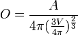
| OVALITY | Ovality. It's calculated by the following equation:
where: O = ovality; A = area; V = volume |
| PLANEANG A1 A2 A3 A4 A5 A6 | Angle between planes defined by A1, A2, A3 and A4, A5, A6. |
| PSA | Polar surface area. |
| RMSD | Calculates the RMSD between the first trajectory frame and the others excluding the hydrogens. |
| RMSDH | As above but including the hydrogens. |
| RMSDALN | Aligns the the first trajectory frame with the others and calculates the RMSD excluding the hydrogens. |
| RMSDALNH |
As above but including the hydrogens. This keyword is equivalent to the old RMSD until the 3.2.2 version. |
| RMSDSYMCOR |
It performs the RMSD calculation without any alignment, but considering the symmetric atoms as equivalent. To do the atom pair selection, the Cahn-Ingold-Prelog (CIP) weights are assigned to each atom and than the hungarian algorithm (also known as Munkres algorithm or Kuhn-Munkres algorithm) is applied to to compute the optimal assignment, minimizing the total cost. |
| RMSDSYMCORH | As above but including the hydrogens. |
| TORSION A1 A2 A3 A4 | Torsion angle. |
| VLOGP | Virtual logP. |
| VOLUME | Molecular volume. |
| VOLDIA | Volume diameter. It's the diameter of a theoretical sphere with the volume of the molecule. |
To select each atom required in the mesure (e.g. A1 A2 etc), you must use the atom number only, or the following syntax: ATOM:RESNAME:RESNUM. RESNAME and RESNUM are optional if ATOM is univocal. Suppose to have a benzene ring and you would like indicate the third atom, like shown in the following PDB file:
...
ATOM 2 C2 BEN 1
-0.695 1.203 -0.002 1.00 0.00
ATOM 3 C3 BEN
1 -1.389 0.000
-0.006 1.00 0.00
ATOM 4 C4 BEN 1
-0.695 -1.203 -0.007 1.00 0.00
...
you can use, without differences, 3 or C3 or C3:BEN or C3:BEN:1. If you want select the atom 482 in a polypeptidic sequence where only one proline is present, you can indicate it with 482 or CA:PRO or CA:PRO:32, but not CA only:
...
ATOM    481  N   PRO    32      -29.658  -2.153   7.524  1.00  0.00
ATOM    482  CA  PRO    32      -28.294  -1.798   7.139  1.00  0.00
ATOM    483  C   PRO    32      -27.169  -2.471   7.908  1.00  0.00
...
ATOM    495  N   VAL    33      -25.978  -2.393   7.325  1.00  0.00
ATOM    496  CA  VAL    33      -24.749  -2.884   7.927  1.00  0.00
ATOM    497  C   VAL    33      -23.841  -1.699   7.661  1.00  0.00
...
If more than one proline is present in this sequence, you can't use CA:PRO neither.
At the end of the property calculation, VEGA shows the ranges, the average value and the standard deviation. If you want exclude the influence of the water in the calculation of dipolar moment, molecular surface, Virtual logP and molecular volume, you can use the -w option.
3.15 -n
This switch enables the normalization of atomic coordinates. The geometry center of a single molecule or a complex is moved to the origin of Cartesian axes.
3.16 -o[OUTPUT]
With -o parameter, you can specify the name of the output file with or without extension. If the filename doesn't have any extension, VEGA automatically adds the appropriate one on the basis of the selected output format (see -f option). The most common extension used by VEGA are shown in the following table:
| Extension | Type | Add | File format |
| .alc | T | Y | Alchemy. |
| .amp | T | Y | AMMP. |
.arc |
T |
N |
Mopac optimized internal coordinates. |
.car |
T |
Y |
Accelrys CAR file (old and new subformat). |
| .cif | T | Y | IUCr Crystallographic Information Framework (CIF/mmCIF). |
| .cml |
T |
Y |
Chemical Markup Language (CML). |
.cor |
T |
Y |
Accelrys CAR file with optimized coordinates. |
.crd |
T |
Y |
CHARMM. |
| .crt | T | A | IUMSC CRT. |
| .cs | T | Y | ChemSol 2. |
.cssr |
T |
Y |
Cambridge Data File (CSSR). |
| .csv | T | Y | Surface in CSV format. |
.dat |
T |
Y |
Mopac cartesian/internal coordinates. |
.dcd |
B |
Y |
CHARMM/NAMD trajectory file. |
.ene |
T |
N |
Accelrys CHARMm energy file. |
.ene |
T |
Y |
VEGA interaction energy file. |
.ent |
T |
N |
PDB. |
.fas |
T |
Y |
FASTA. |
| .fld | T | Y | Tripos COMFA field. |
.gro |
T |
Y |
Gromos/Gromacs. |
.iff |
B |
Y |
Interchange File Format (IFF). |
| .inc | T | N | InChI. |
| .inchi | T | Y | InChI. |
.inf |
T |
Y |
VEGA information file. |
| .inp | T | Y | GAMESS cartesian. |
| .log | T | Y | Gaussian output. |
.ml2 |
T |
Y |
Tripos Sybyl Mol 2. |
| .mol | T | Y | MDL Molfile (V2000), MDL Extended Molfile (V3000). |
.msf |
B |
Y |
MSI Quanta. |
.par |
T |
N |
VEGA parameters. |
.pdb |
T |
Y |
PDB, PDB2, PDBA, PDBF, PDBL and PDBQ. |
| .pdbqt | T | Y | AutoDock 4 / Vina PDBQT. |
| .pqr |
T |
T |
PQR. |
| .psf | T | Y | PSF and PSF X-Plor. |
.qmc |
T |
N |
QMC (CSSR like format). |
| .smi | T |
Y |
Smiles. |
.srf |
B |
Y |
Accelrys Quanta surface. |
.srf |
T |
Y |
Accelrys Insight surface. |
.tem |
T |
N |
VEGA template. |
.wrl |
T |
Y |
VRML (Virtual Reality Markup Language). |
| .xml |
T |
Y |
PQR XML. |
| .xyz | T | Y | CPMD XYZ. |
| .xyz | T | Y | TINKER XYZ. |
.xyz |
T |
Y |
XYZ. |
Where the column Extension is the file extension, Type is
the file type (T = text, B = binary), Add shows if VEGA adds automatically the
extension and File Format is the name of file format.
If you execute VEGA without -o parameter, the output is redirected to the
console (stdout) or to a special device driver (e.g. PRT: for AmigaDOS). This function is
very useful to interface VEGA with another program that can get the input from console.
The redirection is possible with text file formats only.
3.17 -p[FORCE_FIELD]
This function allows to assign the atom types using a specified force field template. This is the most complex function implemented in VEGA. The first challenge being the creation of an universal language, called ATDL (Atom Type Description Language) able to describe virtually any atom type. For more information about ATDL, click here. VEGA uses the force field template files stored in Data directory with the extension .tem (lowercase). The name of these files must be uppercase, but the argument of -p option is case-insensitive. In order to assign the correct atom types, VEGA uses a multiple step algorithm:
Although these steps are very complex, the total process speed is very high.
3.18 -q[METHOD]
Fix the bond order using the specified method that could be: ALL (find the order of all bond) or RINGS (fix the bonds of the aromatic rings making them partial double).
3.19 -r[MODE]
This switch removes the hydrogen atoms: the empty or ALL arguments remove all hydrogens and the APOLAR removes the apolar hydrogens only.
3.20 -s[POINTS]
With this parameter you can change the point density of a surface map. POINTS is the number of points per surface unit (Å2). The default value is stored in the prefs file and usually it is set to 10. For more information about surface calculation, please see the -f[FORMAT] option.
3.21 -t[SECSTRUCT]
The -t option allows to change the protein secondary structure. Two operational mode are available: in the former the user assigns Phi, Psi and Omega torsion values by the syntax TORSION_NAME=value (e.g. Phi=-135), in the latter he put secondary structure name as reported in the following table:
| Sec. structure name | Code | Phi | Psi | Omega | Description |
| AlphaHelix | H | -57.8° | -47.0° | 180.0° | Alpha helix (3,6.13). |
| LeftHelix | L | 57.8° | 47.0° | 180.0° | Left handed alpha helix. |
| 310Helix | 3 | -74.0° | -4.0° | 180.0° | 3.10 helix. |
| PiHelix | P | -57.1° | -69.7° | 180.0° | Pi helix |
| Beta | E | -135.0° | 135.0° | 180.0° | Generic beta strand. |
| BetaAnti | A | -140.0° | 135.0° | 180.0° | Beta strand in anti-parallel sheet. |
| BetaPar | B | -120.0° | 115.0° | 180.0° | Beta strand in parallel sheet. |
Through the keyword PATTERN=, you can set the secondary structure for each residue according the previous table (Code column). If you specify U code, Phi, Psi and Omega are retrieved from the user-defined values set as explained above.
This option can be used to assign the secondary structure when a Fasta file is loading and if it's omitted, the generic beta strand structure is assigned. All sub-parameters are case insensitive.
3.22 -u
This command adds the side chains to a protein. The side chain database is placed in the Data/Fragments directory and it's called Amino acids L.zip. The side chains are added without hydrogens and so, if you need them, you must use the -l option also.
3.23 -v[CPUS]
Set the number of CPUs used in the parallel calculations. The 0 argument means that all installed CPUs are used.
3.24 -w
This switch removes all the water molecules present in an assembly. Please note that VEGA
do not find the water molecules by residue names (e.g. HOH, TIP3, etc), but on the basis
of connectivity table. This approach is slower but more precise and independent of residue
naming.
You can use the -w option in trajectory analysis to neglect the water influence in the
evaluation of dipolar moment, molecular surface and Virtual logP.
3.25 -x[MODE (ID)]
It extracts a molecule from the input database that must be in SDF or ZIP format. The arguments of this options can be:
| Argument 1 | Argument 2 | Description |
| LIST | - | List the name of the molecules in the database. |
| NAME | molecule name | Extract the molecule with the specified name. |
| NUM | molecule number | Extract the molecule with the specified identification number. |
3.26 -y
Find the molecules in the assembly using the connectivity information. This feature is useful when you need to select the molecule (ligand) in the interaction energy evaluation (see -e and -k options), because all file formats, excluding IFF/RIFF, can't store molecule information (starting and ending atoms) in the atom list.
3.27 -z[NTERM CTERM]
Add the capping to N- and C-term position of a peptide when it is built from its primary sequence while is loaded from a FASTA file.
4. Command line examples
vega
show the available options.
vega my_file.car
read my_file.car in Biosym format and print the
converted file in PDB format with connectivity.
vega my_file.cssr.gz -f info
read my_file.cssr.gz, uncompress it and show the molecular
properties.
vega "http://www.rcsb.org/pdb/download/downloadFile.do?fileFormat=pdb&compression=NO&structureId=1QBQ"
-o 1QBQ.iff -f iff
download the molecule from PDB and save it in IFF format.
vega my_file.car -o new_file -b -n
read my_file.car, normalize the coordinates and write new_file.pdb in PDB
format without connectivity, adding .pdb to the output file name.
vega my_file.arc -o new_file.car -f biosym -p cvff
read my_file.arc in Mopac format, assign atom types and write new_file.car in new
Biosym format keeping Mopac charges.
vega file1.pdb file2.dat -o assembly.iff -f iff -w -a
read file1.pdb and file2.dat creating an assembly, remove all water
molecules, renumber the residues and write assembly.iff in Interchange File
Format (IFF).
vega my_file.mol2 -o new_file -p cvff -c gasteiger -f pdbf
translate my_file.mol2 from Tripos Mol2 to PDB Fat format creating new_file.pdb.
The atom types are assigned, using the CVFF force field and the atomic charges, using the Gasteiger method.
vega receptor.car ligand.car -f score -k "BROTO CHARMM36" -d 30 -e 0
calculate the BROTO and CHARMM36 interaction energies between receptor.car and ligand.car with
30 for dielectric constant and shows the results in console. 0
indicates the last molecule in the assembly (ligand.car)
vega my_file.msf -o surface.srf -f QuantaSrf -s 20
calculate the surface accessible to solvent (SAS) using the default probe radius and 20
as point density and save it in surface.srf binary file compatible with Quanta
package.
vega my_file.msf -o surface -f BiosymSrf -g 0
calculate the Van Der Waals surface using default point density and save it
in surface.srf ASCII
file compatible with Insight II package.
vega my_trajectory.CRD -o my_mesure.csv -f csv -m distance
CA:ALA:1 360
analyze a CHARMm trajectory file measuring the distance between two atoms
and storing all data in the my_measure.csv file.
vega my_file.hin -o solvated.pdb -i water 10 sphere
solvate my_file.hin with a spherical water cluster of 10 Å radius.
vega my_file.fas -o my_file_3d.iff -f Iff -t AlphaHelix
load my_file.fas, assign secondary structure as alpha helix and save
it in IFF format.
vega my_file.pdb -o my_file_3d -t phi=-135 psi=135
load my_file.pdb, change the secondary structure and save
it in PDB format, adding the .pdb file extension.
vega my_file.pdb -o my_file -f PDBQT -c Gasteiger -p AutoDock -r
Apolar -j Flex
load my_file.pdb, assign the Gasteiger-Marsili atom charges,
assign the AutoDock atom types, remove the apolar hydrogens, find the
flexible torsion angles and save the molecule in PDBQT format.
vega complex.pdb -o score.xml -f Score -c Gasteiger -e 2 -k "BROTO
ELECT" -y
load assembly.pdb, assign the Gasteiger-Marsili atom charges,
find the molecules, calculate the BROTO (hydrophilic interaction) and
ELECT
(electrostatic interaction) scores, considering as ligand the second molecule in
the assembly and finally save the
results in XML format.
5 Default settings (prefs file)
VEGA (command line) starts reading the preference file in order to set the default parameters. This file is placed in Data directory, it's named prefs and it's in ASCII format editable as a normal text file. Each entry has a keyword with one or more parameters. A semicolon (;) placed in the first column indicates that the line is a remark. Please remember that VEGA doesn't print any warning about incorrect parameters or syntax errors in the prefs file. VEGA ZZ doesn't use this method to set the default parameters. In the following table are shown all available keywords:
| Keyword | Description |
| ENERGY_CONTDIST | Distance used to determine if the ligand is in
contact with a receptor residue (see
-f [FORMAT] option). e.g. ENERGY_CONTDIST 2.5 |
ENERGY_CUTOFF |
Cut-off distance to
speed-up the interaction energy evaluation (see
-f [FORMAT] option). |
ENERGY_DIEL |
Dielectric constant
value (see
-f [FORMAT] option). |
ENERGY_FILTER |
Filter for energy
decomposition by residue (see
-f [FORMAT] option). |
| LANGUAGE | Default language (see
language localization page): |
| MAXATMINFO | It's the maximum atom
number that the info file format (see
-f [FORMAT] option)
can manage for the calculation of extra information. This number is in function of your
CPU power. |
MOPAC_CRG |
Charge attribution with
Mopac keyword CHARGE. It can be set to AUTO (the total charge is calculated by
atomic charges) or to a positive or negative integer value. |
MOPAC_DEF |
Mopac default keywords
(see -k[KEYWORDS] option). |
MOPAC_MMOK |
MMOK is a Mopac keyword
needed to introduce a correction factor when in a molecule there are peptidic
(amidic)
bonds. The argument can be: |
| OCLDEVTYPE |
Set the OpenCL device type. The argument can be: NONE (acceleration disabled), AUTO (automatic detection), DEFAULT (default device), Accelerator (generic accelerator), CPU (generic CPU with SSE3 support) and GPU (Graphic Processing Unit). |
OUTFORMAT |
Output format. |
RENSTART |
Starting residue for
renumbering (see -a [RESNUM]
option). |
SAS_POINTS |
Default point
density for molecular surface calculations (see
-s[POINTS]
). |
SAS_PROBERAD |
Default probe
radius for calculation of the molecular surface accessible to solvent (see
-f [FORMAT] option). |
SOL_RADIUS |
Box length /Sphere
radius / Layer thickness (see -h[SHELL RAD
SHAPE] ). |
SOL_SHAPE |
Shape type (BOX,
SPHERE, SHELL): |
| VOL_DENSITY | Dot density for volume calculations (see -m[KEYWORDS] and -f info ). e.g. VOL_DENSITY 10 |
| XTCPREC | Number of digits after the point (from 1 to 8)
used for the compression of XTC trajectories. e.g. XTCPREC 3 |
For more information about prefs file, see the APPENDIX B.
15. The HyperDrive technology
HyperDrive is a core library including several time-critical functions required by VEGA ZZ for high speed computing. The highly optimized and and parallel code, especially designed for the modern CPUs, allows to speed-up the programs and make faster the development without deep skills in programming. Moreover, the library offers features that are useful not only in developing of molecular modelling software, but also of generic application. In particular, the key features are here summarized:
Hardware independent.
You can develop the same application for Linux (ARM, x86 and x64) and Windows
(x86 and x64) without changes in the source code.
Same software for single or
multiprocessor systems.
The library checks the number of CPUs and automatically switches itself from
sequential to parallel mode.
OpenCL support
Some routines (such as virtual LogP calculation) are written to run on
the GPU thanks to OpenCL abstraction layer.
Simultaneous multithreading (SMT)
ready
It uses the full power of modern multiscalar CPUs with hardware
multithreading such as Intel i5, i6, i9 and AMD Ryzen 5, 7, Threadripper.
Multi core CPU ready
The latest multi core CPUs provided by AMD and Intel are detected and the
parallel execution is automatically enabled.
SIMD optimization
The functions that are more frequently called, are written in assembly and
optimized by using SSE SIMD instruction set.
No special compiler required.
You can use your preferred C/C++ compiler. C++ envelops are included in the
headers.
HyperDrive requires an initialization phase that is executed by the host application when it starts. The host application can choose the appropriate HyperDrive version for the installed microprocessor and the HyperDrive detects the number of CPUs switching itself to run in sequential mode (one CPU) or in parallel mode:
After the initialization phase, the host application can call the HyperDrive functions in transparent mode as a normal library: the HyperDrive library select internally the most appropriate code for that hardware/software system and if it can run more than one thread at the same time at hardware level such as for multicore or SMT CPUs, the code is executed in parallel:
HyperDrive library includes several functions that are shown in the following table according to their application field:
| Molecular modelling functions |
|
|
| Mathematical and statistical functions |
|
|
| Low level |
|
17. Creating a new template
VEGA and VEGA ZZ uses two types of template files: the former is for atom types, and the latter is for atomic charges.
17.1 Force field template
By ATDL (Atom Type Description Language), you can expand VEGA adding new atom types and/or new force field templates. Actually, VEGA supports the following pre-defined templates:
| Force Field | Package |
| AM1BCC | AM1BCC. |
| AMBER | Amber. |
| AUTODOCK | AutoDock 4 force field (based on AMBER). |
| BOND | Used by VEGA to calculate the bond types (single, double, partial double and triple). |
| BROTO | Broto and Moreau atom types for logP calculation. |
| CFF91 | Accelrys CFF91. |
| CHARMM | Accelrys Quanta/CHARMm. |
| CHARMM22_LIG | CHARMM 22 for ligands, including CHARMM22_PRO. |
| CHARMM22_LIPID | CHARMM 22 for lipids. |
| CHARMM22_NA | CHARMM 22 for nucleic acids. |
| CHARMM22_PRO | CHARMM 22 for proteins. |
| CHARMM27 | CHARMM 27 for proteins. |
| CHARMM36_GEN | CHARMM 36 for generic use. The use of this template is not recommended for proteins and nucleic acids. |
| CRIPPEN | Ghose and Crippen atom types for logP calculation. |
| CRIPPEN_MR | Ghose and Crippen atom types for molar refractivity calculation |
| CVFF | Accelrys CVFF. |
| GRID | Grid. |
| GROUPS | Used by VEGA to detect the functional groups. |
| HBOND | H-bond atom types (for internal use). |
| MENG | By Elanie C. Meng and Richard A. Lewis. |
| MM+ | MM+. |
| MM2 | MM2 by N .L. Allinger. |
| MM3 | MM3 by N .L. Allinger. |
| MMFF | MMFF94. |
| OPLS | OPLS. |
| SP4 | Used by VEGA to generate the AMMP input files. |
| TRIPOS | Sybyl by Tripos. |
| UNIV | Used by VEGA to assign the Gasteiger-Marsili atom charges. |
| VINA | AutoDock Vina force field (based on AMBER). |
A force field template is a file storing the atom type descriptions with uppercase name (corresponding to the force field name) and .tem lowercase extension (e.g. AMBER.tem, CVFF.tem, etc). All template files are placed in Data directory. Please remember that the .tem extension is for all VEGA templates and not for force field only.
In all template files the first column can contain special control characters:
| Character | Description |
| ; | Comment marker |
| # | Keyword or command marker |
The first line must contain a keyword needed for file type recognition. For force field it must be:
#TemplateFF [TEMPLATE_NAME] [VERSION]
where TEMPLATE_NAME is the name of the force field template and VERSION is the revision number.
#TemplateFF CVFF 3.0
After this keyword, you can place the atom type description. The first
column is the atom type name (max 8 characters), the second is the atom description in
ATDL and the third contains the description of bonded atoms (also in ATDL).
In this last column, each group of atoms limited by parenthesis contains all atoms bonded
to precedent atom:
C-300 (O-100 O-100)
This line describes a carboxylic carbon: a sp2 carbon bonded to two oxygens making one bond only. More than one levels of parenthesis can be used for complex description of atom types:
C-300 (O-100 O-200 (C-900) C-900)
This line describes a carbonylic carbon of an ester group, bonded to a
generic carbon. The O-200 is also bonded to a generic carbon.
Please remember that VEGA reads the line from left to right and thus the more restrictive
atom description must placed in more left side of line:
C-400 (C-300 X-900 X-900 X-900)
and not:
C-400 (X-900 X-900 C-300 X-900)
If VEGA finds a C-300 as first or second atom bonded to a sp3
carbon, this is recognized as a more generic X-900 atom and can't be reassigned to
the next more specific description.
The description sequence of each atom type goes from more to less specific, from upper to
lower line:
cn	C-400 (N-300 X-900 X-900 X-900) ; more specific
c 	C-400 (X-900 X-900 X-900 X-900) ; less specific
If the order of this two lines is swapped, when VEGA finds a carbon bonded to a sp3 nitrogen, the atom type recognized is a generic c an not a cn.
17.1.1 ATDL atom description
Each atom can be defined by a five character string. The first two characters are the element symbol of atom. If the element symbol is one character only, the second character must be a dash (-). For a better description, special elements can be used:
| Special element | Description |
| X | Any atom. |
| # | Heavy atom (all atoms excluding hydrogens). |
| $ | Any atom excluding carbons and hydrogens. |
| @ | Halogen (F, Cl, Br and I). |
The third character is the bond order: use values from 1 to 6 for real bond order,
0 for non-bonded atom and 9 for a bonded atom with a non-specified bond order.
The fourth character is the ring indicator: use values from 3 to 7 if the atom is a
3 to 7-ring member, 0 for a non-ring member atom and 9 for a non-specified ring atom.
The fifth character is the aromatic indicator: 0 for non-aromatic atom and 1 for
aromatic atom.
The ATDL language allows to use AND, OR and NOT operators (&, | and !) inside a
logical expression included between square.
Examples:
17.2 Atomic charge template
This template file is much different from the first one, because the atom recognition is based on the residue names and the atom names. The control characters are the same of the force field template.
The first line must contain a keyword needed for file type recognition. For force field it must be:
#TemplateCharge [TYPE] [TEMPLATE_NAME]
where TYPE is the template charge type (Gasteiger or
Fragments) and TEMPLATE_NAME is the name of the template. Please remember
that the template name must be the same one of the file without the extension.
Example:
#TemplateCharge Fragments CHARMM22_CHAR
After this keyword it could be present the optional template title/description:
#Title [TEMPLATE_TITLE]
Spaces and special characters are allowed.
Example:
#Title Gasteiger-Marsili charges
After these two keywords, the file can be different if the template type is Gasteiger or Fragments
17.2.1 Gasteiger template
The Gasteiger template is very easy: after the header it's a list of records one for each line. Each record has six fields as reported in the following table:
| Field | Description |
| Type | Atom type. See the UNIV.tem file in the Data directory. |
| a | Gasteiger a parameter. See Tetrahedron, 36, 3219, 1980 and Croat.Chem.Acta, 53, 601, 1980. |
| b | Gasteiger b parameter. |
| c | Gasteiger c parameter. |
| d | Gasteiger d parameter (a + b + c). |
| Charge | Formal charge. |
17.2.2 Fragment template
The fragment template is a little bit complex because it uses some keywords. To define a new residue, you must use the #ResName tag:
#ResName [NAME1] [NAME2] ... [NAME16]
e.g. #ResName ALA ALAN
In this way, you define a new residue that it could have one of the specified names. The maximum number of names is 16 and the maximum length of each name is 4 characters.
This tag could be followed by other optional keywords:
#Id [ID]
e.g. #Id AA_ALA
This command defines an unique residue identificator. It can be used by the #Call command (see below) and its maximum length is 31 characters.
#Description [SHORT_DESCRIPTION]
e.g. #Description Alanine (protonated N-terminus)
It allows to specify a short description for the residue or for the macro (see below). Its maximum size is 127 characters.
#Charge [CHARGE]
e.g. #Charge 1.0
This optional keyword specifies the residue total charge. The number should be a positive or a negative floating point number.
After these optional keywords, that must be after the #ResName tag, the atom section begins. Each atom is defined in a line with the following fields:
[CHARGE] [GROUPID] [BONDS] [NAME1] [NAME2] ... [NAME8]
Where:
| Field | Description |
| CHARGE | Atom partial charge. |
| GROUPID | Group/fragment identification number. It's a positive integer starting from 1 to 255. |
| BONDS | Number of atom bonds. It can be from 0 (non bonded) to 6. If it's greater than 6, the number of bonds isn't checked. |
| NAME1 ... NAME8 |
The atom names. The maximum number of atom names (aliases) is 8 and their maximum length is 4 characters. |
e.g. 0.3100 1 1 HN H H1
This is a complete residue template example:
#ResName ALA
#Id ALA
#Description Alanine
#Charge  0.0000
 -0.4700   1 3 N
  0.3100   1 1 HN   H    H1
  0.0700   1 4 CA
  0.0900   1 1 HA
 -0.2700   2 4 CB
  0.0900   2 1 HB1
  0.0900   2 1 HB2
  0.0900   2 1 HB3
  0.5100   3 3 C
 -0.5100   3 1 O
In red are reported the optional keywords.
In order to simplify the template writing and to make more compact the file size, it's possible to create macros inside the file that must be defined before the use. To begin a new macros, you must use the following command:
#Define [MACROID]
e.g. #Define AMINO_CT
Where the MACROID is the unique identification name of the macro. It have the same function of the #Id command inside the #ResName section. Inside the macro, you can use the #Description, #Call, #Delete commands and the atom records.
#Call [RESIDUEID_OR_MACROID]
e.g. #Call AA_ALA
This command call a residue or a macro executing its commands. It can be placed inside a macro or a residue section.
#Delete [ATOM_NAME]
e.g. #Delete O
This keyword deletes an atom previously defined in a residue section.
Please remember that an atom record inside a macro could replace a previous one if they have the same first atom name. This is a macro example:
#Define AMINO_CT
#Description C-terminus
  0.3400   9 3 C
 -0.6700   9 1 OT1  OCT1 O1   O
 -0.6700   9 1 OT2  OCT2 O2   OXT
#Delete O
Using this macro and an aminoacid residue definition, it's possible to obtain a new one specific for the C-terminal aminoacid:
#ResName ALA ALAC
#Id ALAC
#Description Alanine (negative C-terminal)
#Charge -1.0000
#Call ALA
#Call AMINO_CT
The first call copies the atom definitions from the ALA residue and the second call applies the AMINO_CT macro that change the C atom, add the two carboxyl oxygen, and delete the carbonyl oxygen (O).
19. How-to guide
This section includes some tricks to solve common problems by VEGA ZZ.
19.1 MEP calculation with semi-empirical charges
19.2 Volume calculation
19.3 Trajectory format conversion
19.4 Join two or more trajectory files
19.5 Remove the waters in trajectory files
19.6 Add the side chains to a homology-modelled protein
19.7 AMMP energy minimization
19.8 Installation of Accelrys CHARMM force field
19.9 Conversion of a database to another format
19.1 MEP calculation with semi-empirical charges
19.2 Volume calculation
19.3 Trajectory format conversion
19.4 Join two or more trajectory files
19.5 Remove the waters in trajectory files
19.6 Add the side chains to a homology-modelled protein
19.7 AMMP energy minimization
19.8 Installation of Accelrys CHARMM force field
The Accelrys CHARMM 22 force field allows to do MM/MD calculations of both small and big molecules with less problems than the standard CHARMM force field, because it was expanded with more atom types. For obvious copyright reasons, the ATDL template only (CHARMM.tem) is included in the VEGA ZZ package and not the parameter file (parm.prm), but if you have got an Accelrys software that includes the CHARMm license, you can use it, following this installation procedure:
19.9 Conversion of a database to another format
If you want to convert a database to another format, you need to create a new empty database in the desired format:
20. Frequently Asked Questions
20.1 Generic FAQ
How is it possible to open a NAMD .coor file including atom
properties ?
The NAMD .coor file format includes only the atom coordinates. VEGA ZZ can
open it but the main data of the molecule (atoms, residues, etc) are
missing. To avoid this problem, you can open the file from which the .coor
file was generated (usually a PDB file), thus merge the atom coordinates of
.coor file by selecting File
![]() Merge in the main menu. For more information about the merge
function, click here.
Merge in the main menu. For more information about the merge
function, click here.
Converting PDB into mol2 file the atom
types and the bond orders are incorrect. Why ?
If the PDB file doesn't have the hydrogens, VEGA can't detect the correct atom
hybridization and the Tripos force field is assigned in wrong way. This is not a bug
and the only way to fix this problem is to add the hydrogens before
the conversion.
When I open some PDB files, the
connectivity appears incomplete. Why ?
Starting from VEGA 1.5.0 the PDB CONECT records are read and the
connectivity isn't recalculated if the number of that record is more or
equal to the number of atoms. To solve this problem, you should recalculate the connectivity
for all or for the incomplete atoms, selecting Edit
![]() Add
Add
![]() Bond
from the main menu.
Bond
from the main menu.
When I try to run VEGA on my Linux
RedHat 9 workstation, the message "./vega: relocation error: /usr/local/vega/liblocale.so:
symbol errno, version GLIBC_2.0 not defined in file libc.so.6 with link time
reference" is shown and the program doesn't start. Why ?
This error is due to the introduction of the Native Posix Thread Library (NPTL)
in Red Hat Linux 9.0. Applications complied with older Red Had distributions
(e.g. VEGA and ESCHER NG) are known to experience problems with this library. To work
around this problem, you can use the old Linux threads implementation by
setting the environmental variable LD_ASSUME_KERNEL. Set it to either 2.2.5
or 2.4.1.
If you are using c shell, you can enter one of the following at the LINUX
prompt:
setenv LD_ASSUME_KERNEL 2.4.1
or
setenv LD_ASSUME_KERNEL 2.2.5
If you are using bash shell, you can enter one of the following at the LINUX
prompt:
export LD_ASSUME_KERNEL=2.4.1
or
export LD_ASSUME_KERNEL=2.2.5
Note:
This problem was eliminated starting from the 1.5.7 Linux release.
How many atoms can manage VEGA and
VEGA ZZ ?
In theory, the maximum number of atoms manageable by VEGA is 2^32 =
4.294.967.296. VEGA ZZ can manage this number of atoms for each workspace
and the maximum number of workspaces is 4.294.967.296. These numbers can't
be reached by the 32 bit CPUs because their address space is 32 bit wide
only.
How many atoms can manage Mopac 7
included in VEGA ZZ package ?
VEGA ZZ includes two versions of Mopac 7.01-4: Mopac_50_100.exe (max. 50
heavy atoms and max. 100 hydrogens) and Mopac_100_200.exe (max. 100
heavy atoms and max. 200 hydrogens). The two executables are selected
automatically by VEGA ZZ for a balanced use of the hardware resources.
No more than 300 atoms (100 heavy atoms + 200 hydrogens) can be used by VEGA
ZZ in Mopac calculations.
Can I use trajectory files and
databases with 2 Gb or more sizes ?
Yes. Starting from VEGA ZZ 2.0.2 and VEGA 1.5.3, the io64 library is linked
to the executable allowing to manage files larger than 2 Gb if the file
system permit it: FAT12 has a 16 Mb file size limit, FAT16 has a 2 Gb as its
limit, FAT32 has 4 Gb as its limit but it's reduced to 2 Gb to allow seek
operations. NTFS has a theoretical maximum file size of 16 Exabytes.
The Linux Ext2 file system has a 4 Tb file size limit and the XFS has a
maximum file size of 16 Exabytes.
The Amiga Fast File System (FFS) has a 4 Gb file size limit. This limit is
braked by the Fast File System 2 with a theoretical maximum file size of 16
Exabytes.
Why are the VEGA ZZ 2.0.6+ IFF
files unreadable by previous releases ?
The 2.0.6 release writes the IFF/RIFF files in the native little endian
format (RIFF) by default. The previous releases read the IFF files in big
endian format only and so they are unable to understand the RIFF files. This
isn't a problem, because you can switch from little to big endian checking
Big endian when you save the molecule (File
![]() Save as...).
Please remember that the 64 bit IFF/RIFF files are unreadable by the
previous releases.
Save as...).
Please remember that the 64 bit IFF/RIFF files are unreadable by the
previous releases.
Is it available a soft or a PDF
manual version ?
No, the HTML version is available only. If you want, it's possible to build
a printable version of the manual, clicking on Printable version in the
left summary frame.
Where could I download molecule databases ?
Some institutions allow to access to their own databases for free. For more
information click here.
20.2 VEGA ZZ FAQ
The IFF files generated by VEGA ZZ 3.0.2+ are shown corrupted by the
previous releases. Is it possible to fix the problem ?
Due to the different visualization method implemented in the newer
releases, the IFF files may be shown corrupted by previous releases. To fix
the problem, just press the space bar after loading or update your VEGA ZZ
installation.
How can I open a trajectory file ?
Firstly, the trajectory file must be in any format supported by VEGA ZZ (for
more information, click here). Some trajectory
formats need another file to be opened because they don't contain the
information about atoms, residues, etc, but they include the atom
coordinates only. The formats requiring an extra molecule file are: AutoDock
4 DLG, BioDock 3.0, DCD, ESCHER NG, GROMACS TRR and XTC and Quanta
conformational search .csr.
VEGA ZZ is able to find automatically the required file starting from the
trajectory file name and changing the extension (e.g. my_trajectory.dcd
![]() my_trajectory.pdb). It performs
changes for three times with three different file extensions (e.g. .iff, .pdb
and .crd) that are typical for each trajectory format. If VEGA ZZ can't
find the file, it's unable to read the trajectory. To fix the problem, two
are the possible solutions:
my_trajectory.pdb). It performs
changes for three times with three different file extensions (e.g. .iff, .pdb
and .crd) that are typical for each trajectory format. If VEGA ZZ can't
find the file, it's unable to read the trajectory. To fix the problem, two
are the possible solutions:
- Put in the same directory where is the trajectory, the molecule file with
the same file name prefix of the trajectory (see the example above). VEGA ZZ
can recognize if that file is compatible with the trajectory and if this
condition is not satisfied, an error is shown.
- Open the molecule file (File
![]() Open) that can be in any directory
with any name, then open the trajectory file (Calculate
Open) that can be in any directory
with any name, then open the trajectory file (Calculate
![]() Analysis)
clicking the open button or dragging the file over the trajectory analysis
window.
Analysis)
clicking the open button or dragging the file over the trajectory analysis
window.
For AutoDock 4 DLG, BioDock 3.0 and ESCHER NG, the associated files are
obtained from the record inside the trajectory file. The AutoDock 4 DLG
loader, if doesn't find the file, performs the same procedure
explained above as last chance.
How is the update procedure
?
To update the VEGA ZZ already installed in your system, you must uninstall
it and thus install the new release in the same directory in which was
located the previous one. No new activation is required because the vegazz.lic file isn't removed during the uninstall procedure.
Starting from 3.0 release, VEGA ZZ includes an automatic procedure that
checks periodically the updates. When they are available, the setups are
downloaded from DDL server and installed. The user can perform manually the
update selecting Help
![]() Check for update menu item.
Check for update menu item.
During the installation, Windows reports
this error message: "Error creating registry key and so access is denied". Why ?
The installer writes in the registry the information to uninstall VEGA. No
other data are written. The error is shown if
your user account doesn't have the rights to write the registry. Logon with the
administrator account and re-start the installation procedure.
Why doesn't work the REBOL
scripts in my system ?
With most probability, you installed a software firewall in your PC and
so you must configure it granting the network access to REBOL.exe.
The scripting system needs the access to standard TCP/IP communication
ports.
Why is the REBOL script execution
so slow ?
The REBOL scripts use the TCP/IP port to communicate with VEGA ZZ. This
problem affects Windows 9x and Windows 2000 only. It seems that the TCP/IP
management of these OS has an excessive latency. To increase the TCP/IP
performances try to use the burst commands that reduces the negotiation
time. Windows XP doesn't have this problem and the scripts are executed at
full speed.
When I open file and load the DCD file it
says "no -m option given", but no pull down menu with -m option is present. Why
?
You opened a trajectory file directly from the File
![]() Open menu item. This
procedure is incorrect for the OpenGL operating mode. The correct procedure is the
following:
Open menu item. This
procedure is incorrect for the OpenGL operating mode. The correct procedure is the
following:
- Open the whole molecule from File
![]() Open menu item.
Open menu item.
- Select
Calculate
![]() Analysis.
Analysis.
- Open the trajectory file (click on
the
![]() button).
button).
Starting from the 1.4.0 release, you can open the trajectory file from
File
![]() Open menu item. The associated molecule is loaded automatically without any
request.
Open menu item. The associated molecule is loaded automatically without any
request.
How can I disable a plug-in ?
You can disable a plug-in moving it to
...\Plugins\Win32\Store directory.
VEGA ZZ crashes when it's showing
complex molecules. How can I solve this trouble ?
Use the
OpenGL Setup utility to change the OpenGL
driver from hardware to Microsoft or Mesa 3D .
VEGA ZZ has low 3D performances with
Matrox P-Series graphic cards when the FAA-16x anti aliasing or the stereo
view is enabled. Why ?
These graphic cards use the alpha channel to perform the aliasing reduction
and the stereo view. So, if you open applications that use the alpha key,
the OpenGL performances go down. A common situation is an application that
uses the transparencies to make glass windows (e.g. VEGA, Miranda, WinAmp,
etc). The solution is to disable the glass windows (see the control panel of
the specific application) or to close the program. This problems affects Windows 2000 and
not Windows XP.
How can I improve the graphic
quality ?
If you have an ATI, Matrox P-series, NVIDIA graphic card, enable the anti-aliasing
in the control panel of the display driver. By default, this setting is
disabled. In the OpenGL mode, the Matrox driver supports the 16x anti-aliasing
only.
Enable the vector anti-aliasing in the VEGA ZZ
View
settings window.
How does VEGA add the solvent molecules ?
VEGA uses a pre-calculated solvent cluster placed in
...\VEGA ZZ\Data\Clusters
directory that is a PDB gzipped file. When you add solvent clusters to a
solute, VEGA performs these steps:
- load the solvent cluster;
- move the solute at the centre of the cluster (it have a cubic shape);
- cut the volume occupied by the solute removing the bumping molecules;
- cut the shape as you selected in the graphic interface (box, sphere,
layer).
When you choose Sphere, VEGA cuts a sphere of specified radius
cantered at the barycentre of the solute. When you select Layer, it
cuts the molecules exceeding the distance between them and the closest atom
on the surface. Choosing the Box mode, VEGA cuts the solvent
molecules outside the box user-defined dimensions. The box is cantered at
the barycentre of the solute as for the sphere mode.
This is a generic method for all kinds of solvents. The direction of the
water h-bonds referenced to the solute is not taken in account. For this
reason, after the solvation, you must optimize the system performing an
energy minimization and, eventually, a short molecular dynamics.
20.3 VEGA ZZ activation problems.
I didn't received the
Activation Key because I inserted a wrong e-mail address in the registration
form. How can I change it in order to activate the software ?
The procedure is very easy:
- Connect to DDL license server:
http://www.ddl.unimi.it/licman/login.htm.
- Login with the wrong e-mail address and the password specified during the
registration procedure.
- In the menu, select Update user details and click Go !
- Change the e-mail address and click Update.
- Repeat the activation procedure with the new e-mail address.
- A warning message will be shown, informing you that the Product Key
is already active.
- Request a copy of the Activation Key that will be sent to you at the new
e-mail address.
My Activation Key is lost. Can I
request a copy ?
Yes ! Repeat the activation procedure: a warning message informs you that
your Product Key is already active. Request a copy of it clicking the
link.
I have several PCs and I would like
to install VEGA ZZ on all of them. Can I obtain more than one Activation Key
?
Yes ! There are no limits in the number of activations. Please use the same
e-mail address for all activations to avoid to compile the registration form
each time.
My Activation Key is expired. How
can I obtain a new one ?
Repeat the activation procedure and replace the vegazz.lic file with
the new one sent to you by the activation server.
I received the e-mail with the
Activation Key but I'm unable to open it. Why ?
The Activation Key is a encrypted binary file and VEGA ZZ only is
capable to decrypt and read it. You must follow the activation procedure
reported in the e-mail and in the activation wizard: you must save the
vegazz.lic file in the Data folder placed in the installation
directory. Starting from the 2.0.8 release, if you try to open the
vegazz.lic file, it's automatically copied in the installation directory
and if it's already present, a warning message is shown.
When I try to install the Activation Key, the invalid license file
name message is shown. How can I fix this problem ?
With most probability, you changed the the activation file name from
vegazz.lic to another one or you tried to open it directly from the
e-mail client that decodes it, creating a temporary file that isn't named
correctly.
Try to save the file and double click on it.
Another common problem is due to Windows default setting, hiding the
extension of known files. In particular, if you rename the activation key to
vegazz.lic, the OS keeps the previous .lic extension making
the real file name as vegazz.lic.lic even if vegazz.lic file
name is shown. There are two possible solutions: 1) remove the .lic
file extension; 2) go to the file explorer settings (Folder options
window -> View tab -> Advanced settings list) and uncheck
Hide extensions for known file types.
VEGA ZZ says to me that my system
has an invalid host ID or a CRC error is present in my Key. Few days ago,
the software worked fine. Why ?
Your host ID is changed and this is possible when the hardware network
configuration is changed adding a new network card, modem, IEEE 1394 card
etc or updating the motherboard BIOS and/or device drivers. In this
situation, the solution is repeat the activation procedure.
It's possible to create an Activation Key for a computer not connected
to Internet ?
Yes, it's possible following this procedure:
NC is the PC not connected to Internet.
C is the PC connected to Internet.
- Download VEGA ZZ with C.
- Transfer the package from C to NC (e.g. by pen drive, CD, etc).
- Install the package on NC and start VEGA ZZ. The activation wizard will be show.
- Annotate the Product Key. Please remember that it's not the same of C.
- Start Internet Explorer in C and connect to http://www.ddl.unimi.it/licman.
- Put the Product Key of NC, your e-mail address and complete the activation as usual.
- When you receive the e-mail with the vegazz.lic file, transfer it to NC and copy it un the ...\VEGA ZZ\Data directory. VEGA ZZ on NC is now operative.
22. Bugs
VEGA ZZ and VEGA are pieces of software with many functions, therefore it might be possible to discover minor bugs.
22.1 Bug report
VEGA ZZ 3.0 contains a built-in bug report utility called madExcept that help you to send the data needed by us to identify and fix the problem. If a serious error occurs, this dialog window is shown:
in which it's possible to choose different actions:
changing the tabs, its possible to show the data that will be sent to us;
Complete the form typing your name and your e-mail address, check remember me if you want save your contact information and click Continue.
Explain the situation in which the error occurs and click Continue or Skip if you have nothing to explain.
Clicking Continue, the report will be sent to us. Please note that no sensitive personal information will be sent to us and all data will be used for debug purpose only.
If you find a non-critical bug not showing the report utility you can contact
us by this e-mail address:
bugreport@vegazz.net.
For other questions please refer to the
Authors address in copyright section.
22.2 Known bugs
22.2.1 Amiga version
The powerpacker.library accepts only standard Amiga DOS paths and not Unix-like syntax of ixemul.library. The Data Decompressor Engine shows an error (file not found) if a file is powerpacked and the path has the Unix-like syntax.
The HyperDrive library is statically linked and it doesn't support symmetrical multiprocessing and OpenCL.
22.2.2 VEGA ZZ
Using multi-monitor systems (e.g. dual head graphic cards or two graphic cards) under Windows 9x/ME, the 3D hardware acceleration is not available. This is not a VEGA bug, but a limit of the Microsoft operating system. Windows 2000/XP don't have this problem.
When the monitor in suspend mode is waked up, the double buffer of the main window could be corrupted. You must force the refresh, minimizing and restoring the main window.
When you save an image using the hardware rendering and you installed a Matrox P-Series graphic card, the labels aren't rendered. This is a bug in the Matrox OpenGL driver: the switching of the device context is not detected. The rendering with the software driver (provided by Microsoft) works fine.
The PDF, PostScript, EPS and LaTex drivers don't support transparencies and smoothed vectors.
See the compatibility list for the graphic accelerators.
23. Development information
The VEGA package was originally developed to run with AmigaOS using its graphic interface. The GUI was totally rewritten to work with all Windows systems and takes the advantages of the OpenGL graphic API.
23.1 Hardware for beta testing
In this section, you can find the hardware platforms used to develop and test VEGA and VEGA ZZ:
PC IBM compatible: AMD Ryzen 9 3900X 12 core 3.8 GHz, Windows 10 Professional x64, 32 Gb DDR4 Ram, NVIDIA GeForce RTX 2070 Super 8 Gb DDR6 PCIe card, HTC Vive Pro Eye HMD, 512 Gb NVMe SSD, 6.0 Tb 7.200 rpm HD, SATA DVD-Writer, 10/100/1000 Ethernet card.
Asus RS700-E7/RS8 Intel: 2 Intel Xeon E5-2620 eight core 2.0 GHz, CentOS 6.2/Windows 7 Professional x64, 64 Gb DDR3 Ram, Aspeed AST2300 16MB VRAM, 3x 500 Gb SATA-2 7.200 rpm HDs, DVD-Writer, 4x 10/100/1000 Ethernet cards.
PC IBM compatible: AMD Phenom II X6 1090T six core 3.2 GHz, Windows 7 Professional x64, 8 Gb DDR3 Ram, Sapphire/ATI HD5770 1 Gb DDR5 PCIe card, 512 Gb SSD SATA-3, 2x500 Gb 7.200 rpm SATA HDs, SATA BD-Writer, SATA DVD-Writer, 10/100/1000 Ethernet card.
23.2 Development tools
No endorsement of any hardware of software should be inferred
24. History
- Calculation\XLOGP2.
calculate the logP by XLOGP V2 method.
- Database\SMILES to database.c
convert a file containing SMILES strings to a database.
- Docking\PLANTS\Rescore ChemPlp.c
- Docking\PLANTS\Rescore Plp.c- Docking\PLANTS\Rescore Plp95.c
evaluate ligand - receptor interactions by different PLANTS scoring functions.
- Docking\Vina\Docking.c
Vina graphic interface.
- Docking\Vina\Ligand.c
prepare the ligand to be docked by Vina.
- Docking\Vina\Receptor.c
prepare the receptor to be docked by Vina.
- Docking\Vina\Virtual screening.c
complete easy-to-use virtual screening system based on Vina.
- Docking\X-Score.c
evaluate ligand - receptor interactions by X-Score.
- Interaction surface\CHARMM interaction surface.c
show the ligand-receptor interaction surface using the CHARMM force field.
- Interaction surface\Lipophilic interaction surface.c
show the ligand-receptor lipophilic interaction surface.
- Interaction surface\MEP interaction surface.c
show the ligand-receptor electrostatic interaction surface).
- Interaction surface\MLPInS color ramp.c
normalize the color ramp of surfaces calculated by MLPInS interaction surfaces.c
- Interaction surface\MLPInS interaction surfaces.c
show the ligand-receptor MLPInS interaction surface
- Movie\Sec. structure anim.c
create a movie changing the secondary structure.
- QSAR\Automatic linear regression.c
generate all possible regression models.
- QSAR\Linear regression.c
perform multiple linear regressions.
- Trajectory\DCD fix for VMD.c
patch buggy DCD files generated by pre-3.0.0 VEGA ZZ releases.
- New batch files: Namd.cmd (NAMD command line interface), NamdClean.cmd (clean the directory removing useless files and keeping NAMD results), NamdMulti.cmd (perform multiple NAMD calculations considering all input files in a given directory).
- AutoDock 4 and AutoGrid 4 were compiled by gcc 4.6.3 for x86 and x64 Windows with a significant performance improvement (from 2 to 3 time faster than the previous build made by gcc 3.4.5).
- AutoDock Vina 32 and 64 bit version built by gcc 4.6.3 are now included in the package. Vina 64 bit is up to two time faster than the original 32 bit version.
- gcc and gfortran 4.6.3 were used to update both 32 and 64 bit executables (AMMP, ChemSol2, ESCHER NG, Fpocket, HyperDrive, InChI, Mopac7, Predator, PropKa, VEGA command line).
- Updated gl2ps library to 1.3.6.
- Updated InChI library to 1.03.
- Updated REBOL to 2.7.8.
- VEGA ZZ in now compiled by RAD Studio XE.
- Support of Wine emulation layer discontinued.
- VEGA command line for Linux includes binaries for both x86 (32 bit) and x64 (64 bit) operating systems in a unique package. Now, the same package contains also: AMMP, ESCHER NG, GriDock, Mopac 7 and SQLite.
26. How to cite VEGA and VEGA ZZ
If you use VEGA and VEGA ZZ for your research, you agree to cite the publications detailing the original methods and reference data used, as well as one of the specific papers:
A. Pedretti, A. Mazzolari, S. Gervasoni, L. Fumagalli, G. Vistoli
"THE VEGA SUITE OF PROGRAMS: AN VERSATILE PLATFORM FOR CHEMINFORMATICS AND DRUG DESIGN PROJECTS"
Bioinformatics, Vol. 37(8) 1174-1175 (2021).
DOI: 10.1093/bioinformatics/btaa774
Other articles on VEGA an related programs are available here.
Electronic documents should include a direct link to the Drug Design Lab home page:
http://www.ddl.unimi.it
or to VEGA ZZ Web site:
http://www.vegazz.net
27. Acknowledgements
Special thanks to all VEGA testers:
All people unintentionally not mentioned in this document, please don't offend.
No endorsement of any hardware of software should be inferred
APPENDIX A - Gasteiger-Marsili parameters
All this parameters are included in GASTEIGER.tem file stored in Data directory.
#TemplateCharge Gasteiger

; *************************************************
; ****              VEGA Template              ****
; ****  Gasteiger-Marsili template for charges ****
; *************************************************

; Ref. Tetrahedron, 36, 3219, 1980
;      Croat.Chem.Acta, 53, 601, 1980

#Title Gasteiger-Marsili charges

; Type        a        b        c        d      Charge
; =====================================================
  H          7.17     6.24    -0.56    12.85     0.000000
  HOS3      15.00     6.24    -0.56    20.68     0.000000
  C3         7.98     9.18     1.88    19.04     0.000000
  C2         8.79     9.32     1.51    19.62     0.000000
  CS2        7.35     1.40     0.30     8.40     0.000000
  C1        10.39     9.45     0.73    20.57     0.000000
  N3        11.54    10.82     1.36    23.72     0.000000
  N2        12.87    11.15     0.85    24.87     0.000000
  N1        15.68    11.70    -0.27    27.11     0.000000
  O3        14.18    12.92     1.39    28.49     0.000000
  O2        17.07    13.79     0.47    31.33     0.000000
  OS4E      13.00     5.00     1.50    18.00     0.000000
  F         14.66    13.85     2.31    30.82     0.000000
  Cl        11.00     9.69     1.35    22.04     0.000000
  Br        10.08     8.47     1.16    19.71     0.000000
  I          9.90     7.96     0.96    18.82     0.000000
  S2        10.50     1.80     2.00    13.80     0.000000
  S3        10.14     9.13     1.38    20.65     0.000000
  P          8.90     8.32     1.58    18.10     0.000000
  Du         0.00     0.00     0.00     1.00     0.000000
  SO2        7.00     1.40     0.30     8.40     0.000000
  SO4        5.40     1.40     0.30     6.40     0.000000
  OS2       18.00     2.00     0.20    20.00     0.000000
  CSO2      12.00     1.80     2.00    13.80     0.000000
  NSO2      13.00     1.80     2.00    14.80     0.000000

; Atoms with localized partial charge
  CN        10.39     9.45     0.73    20.57    -0.500000
  S-        10.14     9.13     1.38    20.65    -1.000000
  SO1       10.14     9.13     1.38    20.65     1.000000
  S+         5.10     3.80     0.50    20.65     1.000000
  SO3H       5.14     5.13     0.38    10.65     3.000000
  SO3-       5.14     5.13     0.38    10.65     2.000000
  NC        15.68    11.70    -0.27    27.11    -0.500000
  O-        17.07    13.79     0.47    31.33    -0.500000
  OP        17.07    13.79     0.47    31.33    -0.500000
  OP=       17.07    13.79     0.47    31.33    -0.666667
  OS1       17.07    13.79     0.47    31.33    -1.000000
  OS3       17.07    13.79     0.47    31.33    -1.000000
  OS4       17.07    13.79     0.47    31.33    -0.333334

; Guanidine group:
  CG         8.79     9.32     1.51    19.62     0.040000
  NG        17.07    13.79     0.47    31.33     0.320000

  N3+       11.54    10.82     1.36    23.72     1.000000
  NP+       11.54    10.82     1.36    23.72     1.000000
  NI+       11.54    10.82     1.36    23.72     0.500000

  PN        11.54    10.82     1.36    23.72     0.000000
  P=         8.90     8.32     1.58    18.10     0.010000

  Na         0.00     0.00     0.00     1.00     1.000000
  K          0.00     0.00     0.00     1.00     1.000000
  Ca         0.00     0.00     0.00     1.00     2.000000
  Mg         0.00     0.00     0.00     1.00     2.000000
  Mn         0.00     0.00     0.00     1.00     2.000000
  Fe         0.00     0.00     0.00     1.00     2.000000
  Zn         0.00     0.00     0.00     1.00     2.000000
  Co         0.00     0.00     0.00     1.00     3.000000
  Cr3+       0.00     0.00     0.00     1.00     3.000000
  F0         0.00     0.00     0.00     1.00    -1.000000
  Cl0        0.00     0.00     0.00     1.00    -1.000000
  Br0        0.00     0.00     0.00     1.00    -1.000000
  I0         0.00     0.00     0.00     1.00    -1.000000
APPENDIX B - VEGA prefs file
This is an example of VEGA prefs file. This file must be placed
in Data directory.
; ********************************************
; ****      VEGA V3.2.3 - Preferences     ****
; **** (c) 1997-2023, Alessandro Pedretti ****
; ****         All rights reserved        ****
; ********************************************

; This file can be changed manually with a text editor. No errors will be
; displayed by VEGA loading the configuration. All fields are case-insensitive.


; **** General preferences ****
;
; Language:
; (ignored by AmigaOS)

LANGUAGE        Auto

; Default output format:

OUTFORMAT	PDB2

; Overlapping tolerance for connecctivity calculation (%)

CONNTOL         20.0

; Starting residue for renumbering:

RENSTART	1

; **** Interaction energy calculation ****
;
; Contact distance for score calculation

ENERGY_CONTDIST 2.5

; Cutoff distance (Amstrong):

ENERGY_CUTOFF	10.0

; Filter for energy decopmosition by residue (%):

ENERGY_FILTER	1.0

; Dielectric constant:

ENERGY_DIEL	1

; **** Info format ****
;
; Max atom number for calculation of extra information:
; Surface, volume, logP, etc.

MAXATMINFO      5000

; **** Mopac format ****
;
; Default keywords:

MOPAC_DEF	AM1 PRECISE GEO-OK

; Charge calculation (AUTO/charge):

MOPAC_CRG	AUTO

; Peptide bond correction (AUTO/ON/OFF):

MOPAC_MMOK	AUTO

; **** SAS parameters ****
;
; Probe radius (A):

SAS_PROBERAD	1.4

; Dot density:

SAS_POINTS	10

; **** Shell generation ****
;
; Box length / Sphere radius / Shell (A):

SOL_RADIUS	10.0

; Shape type (Box, Sphere, Shell):

SOL_SHAPE	BOX

; **** Volume calculation ****
;
; Dot density for cubic Angstrom

VOL_DENSITY     12

; **** HyperDrive parameters ****
;
; Number of CPUs used by HyperDrive (0 = all installed CPUs)

MAXCPU              0
; **** OpenCL ****
;
; Device type:
; None = OpenCL disabled
; Auto = Automatic detection
; Default = default device
; Accelerator = generic accelerator (e.g. IBM Cell Broadband Engine)
; CPU = generic CPU with SSE3 support (specific driver required)
; GPU = Graphic Processing Unit
;
; For the CPU device, a specific driver must be installed (e.g. included in the
; AMD Stream package).

OCLDEVTYPE         Auto
; **** XTC compression ****
;
; Number of digits after the point (from 1 to 8)

XTCPREC 3
APPENDIX C - CVFF atom types
The CVFF.tem file is stored in Data directory.
#TemplateFF CVFF 3.0

; ******************************
; ****  VEGA Template V4.0  ****
; ****   Force Field CVFF   ****
; ******************************


; ATDL atom description:
; ~~~~~~~~~~~~~~~~~~~~~~
; Element (2) - Bond order (1) - Ring indicator (1) - Aromatic indicator (1)
;
; The brackets indicates the length in characters of each field.

; Generic elements:                     Bond order:
; ~~~~~~~~~~~~~~~~~                     ~~~~~~~~~~~
; X = Any atom                          0   = Atom not bonded
; # = Heavy atom                        1-6 = Bond order
; $ = Any atom excluding C and H        9   = Any bond order
; @ = Halogen
; - = None

; Ring indicator:                       Aromatic indicator:
; ~~~~~~~~~~~~~~~                       ~~~~~~~~~~~~~~~~~~~
; 0     = Don't check ring              0 = Don't check
; 2     = Not inside a ring             1 = Aromatic
; 3...7 = From 3 to 7 member ring
; 9     = Generic ring

; Logical operators:
; ~~~~~~~~~~~~~~~~~~
; to use the logical operators AND, OR and NOT (&, | and !), you must
; place the expression between square brackets at the specified position:
;
; Examples:
; [C- |  N-]900  -> the element can be carbon or nitrogen
; [X- & !Cl]900  -> all elements but not chlorine
; C-[4 | 3]00    -> sp3 or sp2 carbon
; C-4[9 & 9]0    -> sp3 carbon in a double condensed ring
; C-3[6 | 5][!1] -> sp2 carbon in 5 or 6 member ring not aromatic

; Atom types:
; ~~~~~~~~~~~
; each not blank and not commented line (; is the remark indicator) must
; include at least the atom type name (max. 8 characters) and the ATDL
; description. Optionally, you can specify the bonded atoms placing them
; between round brackets.


; Type    Atm    Bonded atoms
; ========================================================================; ATDL atom description:
; ~~~~~~~~~~~~~~~~~~~~~~
; Element (2) - Bond order (1) - Ring indicator (1) - Aromatic indicator (1)
;
; The brackets indicates the length in characters of each field.

; Generic elements:                     Bond order:
; ~~~~~~~~~~~~~~~~~                     ~~~~~~~~~~~
; X = Any atom                          0   = Atom not bonded
; # = Heavy atom                        1-6 = Bond order
; $ = Any atom excluding C and H        9   = Any bond order
; @ = Halogen
; - = None

; Ring indicator:                       Aromatic indicator:
; ~~~~~~~~~~~~~~~                       ~~~~~~~~~~~~~~~~~~~
; 0     = Don't check ring              0 = Don't check
; 2     = Not inside a ring             1 = Aromatic
; 3...7 = From 3 to 7 member ring
; 9     = Generic ring

; Logical operators:
; ~~~~~~~~~~~~~~~~~~
; to use the logical operators AND, OR and NOT (&, | and !), you must
; place the expression between square brackets at the specified position:
;
; Examples:
; [C- |  N-]900  -> the element can be carbon or nitrogen
; [X- & !Cl]900  -> all elements but not chlorine
; C-[4 | 3]00    -> sp3 or sp2 carbon
; C-4[9 & 9]0    -> sp3 carbon in a double condensed ring
; C-3[6 | 5][!1] -> sp2 carbon in 5 or 6 member ring not aromatic

; Atom types:
; ~~~~~~~~~~~
; each not blank and not commented line (; is the remark indicator) must
; include at least the atom type name (max. 8 characters) and the ATDL
; description. Optionally, you can specify the bonded atoms placing them
; between round brackets.


; Type    Atm    Bonded atoms
; ========================================================================

  h    H-100  (C-900)
  h+   H-100  (N-400)
  hn   H-100  (N-900)
  h*   H-100  (O-200 (H-100 H-100))
  ho   H-100  (O-900)
  hp   H-100  (P-900)
  hs   H-100  (S-900)
  dw   D-100  (O-200 (D-100 H-100))
  dw   D-100  (O-200 (D-100 D-100))
  d    D-100  (X-900)

  c3h  C-430  (C-430 H-100 H-100 #-930)
  c3m  C-430  (C-430 #-930 X-900 X-900)
  c4h  C-440  (H-100 H-100 X-940 X-940)
  c4m  C-440  (X-940 X-940 X-900 X-900)
  cg   C-400  (N-400 (H-100 H-100) C-300 H-100 H-100)
  cg   C-400  (N-300 (H-100) C-300 H-100 H-100)
  ca   C-400  (N-400 C-300 H-100 X-900)
  ca   C-400  (N-300 C-300 H-100 X-900)
  coh  C-400  (O-200 (C-900) O-200 H-100 X-900)
  co   C-400  (O-200 (C-900) O-200 X-900 X-900)
  c3   C-400  (H-100 H-100 H-100 X-900)
  c2   C-400  (H-100 H-100 #-900 #-900)
  c1   C-400  (H-100 #-900 #-900 #-900)
  cn   C-400  (N-400 X-900 X-900 X-900)
  cn   C-400  (N-300 X-900 X-900 X-900)
  c    C-400  (X-900 X-900 X-900 X-900)
  ci   C-351  (N-351 (H-100) N-351 (H-100) X-900)
  cs   C-351  (S-251 X-951 X-900)
  c5   C-351  (X-951 X-951 X-900)
  cp   C-391  (X-991 X-991 X-900)
  cr   C-300  (N-300 N-300 N-300)
  cr   C-300  (N-200 N-300 N-300)
  c'   C-300  (O-100 N-300 X-900)
  c-   C-300  (O-100 O-100 X-900)
  c"   C-300  (O-100 X-900 X-900)
  c=   C-300  (X-900 X-900 X-900)
  ct   C-200  (X-900 X-900)

  n4   N-400  (X-900 X-900 X-900 X-900)
  ni   N-351  (C-351 (N-351) C-351 H-100)
  np   N-391  (X-991 X-991)
  no   N-300  (O-100 O-100)
  n1   N-300  (C-300 (N-300 N-300) C-400 H-100)
  n2   N-300  (C-300 (N-300 N-900) H-100 H-100)
  n    N-300  (C-300 (O-100) X-900 X-900)
  n3   N-300  (X-900 X-900 X-900)
  np   N-291  (X-991 X-991)
  n=   N-200  (X-900 X-900)
  nt   N-100  (X-900)

  o*   O-200  (H-100 H-100)
  oh   O-200  (H-100 X-900)
  o-   O-200  (Mg900 C-900)
  o-   O-200  (Zn900 C-900)
  o    O-200  (X-900 X-900)
  o-   O-300  (Mg900 Mg900 C-900)
  o-   O-100  (C-300 (O-100 O-100))
  o-   O-100  (P-400)
  o'   O-100  (C-300)
  o'   O-100  (N-300 (O-100 O-100))
  o'   O-100  (S-400)
  oo   O-900  (O-900 Fe900)

  s    S-400
  sh   S-200  (H-100 C-900)
  s    S-200  (C-900 X-900)
  s1   S-200  (S-200 X-900)
  s    S-100

  p    P-900
  si   Si900

  f    F-100  (C-900)
  cl   Cl100  (C-900)
  Cl   Cl000
  br   Br100  (C-900)
  Br   Br000
  i    I-900

  ar   Ar000
  Na   Na000
  c+   Ca000
  c+   Mg900
  cu   Cu900
  fe   Fe900
  pt   Pt900
  Zn   Zn900

  nu   Nu900
APPENDIX C - TRIPOS atom types
The TRIPOS.tem file is stored in Data directory and it contains the new atom types with more than four character length.
#TemplateFF TRIPOS 3.1

; ******************************
; ****  VEGA Template V4.0  ****
; ****  Force Field TRIPOS  ****
; ******************************


; ATDL atom description:
; ~~~~~~~~~~~~~~~~~~~~~~
; Element (2) - Bond order (1) - Ring indicator (1) - Aromatic indicator (1)
;
; The brackets indicates the length in characters of each field.

; Generic elements:                     Bond order:
; ~~~~~~~~~~~~~~~~~                     ~~~~~~~~~~~
; X = Any atom                          0   = Atom not bonded
; # = Heavy atom                        1-6 = Bond order
; $ = Any atom excluding C and H        9   = Any bond order
; @ = Halogen
; - = None

; Ring indicator:                       Aromatic indicator:
; ~~~~~~~~~~~~~~~                       ~~~~~~~~~~~~~~~~~~~
; 0     = Don't check ring              0 = Don't check
; 2     = Not inside a ring             1 = Aromatic
; 3...7 = From 3 to 7 member ring
; 9     = Generic ring

; Logical operators:
; ~~~~~~~~~~~~~~~~~~
; to use the logical operators AND, OR and NOT (&, | and !), you must
; place the expression between square brackets at the specified position:
;
; Examples:
; [C- |  N-]900  -> the element can be carbon or nitrogen
; [X- & !Cl]900  -> all elements but not chlorine
; C-[4 | 3]00    -> sp3 or sp2 carbon
; C-4[9 & 9]0    -> sp3 carbon in a double condensed ring
; C-3[6 | 5][!1] -> sp2 carbon in 5 or 6 member ring not aromatic

; Atom types:
; ~~~~~~~~~~~
; each not blank and not commented line (; is the remark indicator) must
; include at least the atom type name (max. 8 characters) and the ATDL
; description. Optionally, you can specify the bonded atoms placing them
; between round brackets.


; Type    Atm    Bonded atoms
; ========================================================================

  H.t3p  H-100 (O-200 (H-100 H-100))
; H.spc  H-100 (O-200 (H-100 H-100))
  H      H-100

  C.3    C-400
  C.ar   C-391
  C.cat  C-300 (N-300 N-300 N-300)
  C.2    C-300
  C.1    C-200

  N.4    N-400
  N.ar   N-391
  N.am   N-300 (C-300 (O-100))
  N.pl3  N-300 (C-300)
  N.3    N-300
  N.ar   N-291
  N.2    N-200
  N.1    N-100

  O.t3p  O-200 (H-100 H-100)
; O.spc  O-200 (H-100 H-100)
  O.3    O-200
  O.ar   O-291
  O.co2  O-100 (C-300 (O-100 O-100))
  O.co2  O-100 (P-400 (O-100 O-100 O-100))
  O.2    O-100

  S.3    S-400 (Lp100 Lp100)
  S.O2   S-400 (O-100 O-100)
  S.O    S-300 (O-100)
  S.3    S-200
; S.ar   S-291
  S.2    S-100

  P.3    P-400

  I      I-100
  I      I-000
  F      F-100
  F      F-000
  Cl     Cl100
  Cl     Cl000
  Br     Br100
  Br     Br000

  Se     Se900
  Si     Si400

  Na     Na900
  K      K-900
  Ca     Ca900
  Mg     Mg900
  Li     Li900
  Al     Al900
  Fe     Fe900
  Mn     Mn900
  Mo     Mo900
  Co.oh  Co900
  Cr.th  Cr300
  Cr.oh  Cr600
  Zn     Zn900
  Sn     Sn900

  Du     Du900
  LP     Lp900

  Hev    #-900
  Any    X-900
APPENDIX C - UNIV atom types
The UNIV.tem file is stored in Data directory.
#TemplateFF UNIV 1.0

; ******************************
; ****  VEGA Template V3.0  ****
; ****   UNIV atom types    ****
; ******************************


; NOTE:
; This template is expecially designed for Gasteiger-Marsili charge template and
; can't be renamed or removed. It's based on MENG atom type definitions.

; Description:
; ~~~~~~~~~~~~
; Generic atom type - Bond order - Ring indicator - Aromatic indicator

; Generic atom types:                   Bond order:
; ~~~~~~~~~~~~~~~~~~~                   ~~~~~~~~~~~
; X = Any atom                          0   = Atom not bonded
; # = Heavy atom                        1-6 = Bond order
; $ = Any atom excluding C and H        9   = Any bond order
; @ = Halogen
; - = None

; Ring Indicator:                       Aromatic Indicator:
; ~~~~~~~~~~~~~~~                       ~~~~~~~~~~~~~~~~~~~
; 0     = Don't check ring              0 = Don't check
; 3...6 = From 3 to 6 member ring       1 = Aromatic
; 9     = Generic ring


; Type Atm    Bonded Atoms
; ========================================================================
  HOS3 H-100 (O-200 (S-400))
  H    H-100

  CSO2 C-400 (S-400 (O-100 O-100 N-900 C-900))
  CSO2 C-400 (S-400 (O-100 O-100 C-900 C-900))
  C3   C-400
  CSO2 C-300 (S-400 (O-100 O-100 N-300 C-900))
  CSO2 C-300 (S-400 (O-100 O-100 C-900 C-900))
  CS2  C-300 (S-100 C-900 C-900)
  CG   C-300 (N-300 N-300 N-300)
  C2   C-300
  C1   C-200
  CN   C-100 (N-100)

  N3+  N-400
  N3   N-361 (C-361 (O-100) C-361)
  NP+  N-361
  NI+  N-351 (C-351 (N-351 N-351))
  NG   N-300 (C-300 (N-300 N-300 N-300))
  NSO2 N-300 (S-400 (O-100 O-100 N-300 C-900))
  N3   N-300
  N2   N-200
  NC   N-100 (C-100)
  N1   N-100

  O3   O-200  (P-400 P-400)
  O3   O-200  (P-400 C-900)
  OP   O-200  (P-400 (O-200 O-200 O-100 O-100))
  OS4E O-200  (S-400 (O-100 O-100 O-200 O-900))
  OS1  O-200  (S-400 H-100)
  O-   O-200  (C-300 Zn900)
  O3   O-200

  O3   O-100  (S-400 (O-100 O-100 O-200 (C-900) C-900))
  OS4  O-100  (S-400 (O-100 O-100 O-100 O-900))
  OS3  O-100  (S-400 (O-100 O-100 O-100 C-900))
  OS2  O-100  (S-400 (O-100 O-100 C-900 C-900))
  OS2  O-100  (S-400 (O-100 O-100 N-300 C-900))
  OS1  O-100  (S-400)
  OS1  O-100  (S-300)
  O-   O-100  (C-300 (O-100 O-100))
  OP   O-100  (P-400 (O-200 O-200 O-100 O-100))
  OP   O-100  (P-400 (O-200 N-300 O-100 O-100))
  OP=  O-100  (P-400 (O-100 O-100 O-100))
  O2   O-100

  SO4  S-400  (O-100 O-100 O-900 O-900)
  SO3H S-400  (O-200 (H-100) O-100 O-100)
  SO3- S-400  (O-100 O-100 O-100 C-900)
  SO2  S-400  (O-100 O-100 C-900 #-900)
  SO1  S-300  (O-100 C-900 C-900)
  S+   S-300
  S-   S-200  (C-400 Zn900)
  S3   S-200
  S-   S-100  (C-400)
  S-   S-100  (C-350 (N-250 S-250))
  S2   S-100  (C-300)
  S2   S-100  (C-200)
  PN   P-400  (O-200 O-200 O-100 O-100)
  P=   P-400  (O-100 O-100 O-100)
  P    P-900

  F0   F-000
  Cl0  Cl000
  Br0  Br000
  I0   I-000

  F    F-900
  Cl   Cl900
  Br   Br900
  I    I-900

  Na   Na900
  K    K-900
  Ca   Ca900
  Mg   Mg900
  Mn   Mn900
  Co   Co900
  Cr3+ Cr000
  Fe   Fe900
  Zn   Zn900

  Du   X-900
APPENDIX D CSV Surface Format
The CSV Surface Format is a simple Comma Separated Values (CSV) file in which the field separator is the semicolon character (;) and uses the following format:
12345678901234567890123456789012345678901234567890123456789012345678901234567890123456789
NNNNNN; XXXXXX.XXXXXXXX; YYYYYY.YYYYYYYY; ZZZZZZ.ZZZZZZZZ; VVVVVV.VVVVVVVV; RRR; GGG; BBB

NNNNNN          <- Number of the atom associated to the surface dot (C: %6d, Fortran: i6)
XXXXXX.XXXXXXXX <- X coordinate (C: %15.8f, Fortran: f15.8)
YYYYYY.YYYYYYYY <- Y coordinate (C: %15.8f, Fortran: f15.8)
ZZZZZZ.ZZZZZZZZ <- Z coordinate (C: %15.8f, Fortran: f15.8)
VVVVVV.VVVVVVVV <- Property value projected to the surface dot  (C: %15.8f, Fortran: f15.8)
RRR             <- Red component of the dot color (C: %3d, Fortran: i3)
GGG             <- Green component of the dot color (C: %3d, Fortran: i3)
BBB             <- Blue component of the dot color (C: %3d, Fortran: i3)
Example:
...
    19;      6.75958252;      1.91035986;      1.95385861;      0.00207091;   0;   0; 255
    19;      7.02752399;      2.00558615;      1.95385861;     -0.00113359;  47; 255;   0
    19;      7.08981323;      4.05955124;      1.76369834;      0.00192202;  87; 255;   0
    19;      6.82545519;      4.15205383;      1.76369834;      0.00394259; 113; 255;   0
    19;      6.82545519;      1.71330953;      1.76369834;     -0.00801759;   0; 255;  42
    19;      6.82479095;      4.32851887;      1.54213154;     -0.00837863;   0; 255;  47
    19;      6.54714155;      4.35586500;      1.54213154;     -0.00651778;   0; 255;  23
    19;      6.26949215;      4.32851887;      1.54213154;     -0.00380767;  12; 255;   0
    19;      6.00251293;      4.24753141;      1.54213154;     -0.00061359;  53; 255;   0
    19;      5.75646353;      4.11601543;      1.54213154;      0.00250929;  94; 255;   0
...
    48;      6.40636539;      3.02671599;      2.81072426;      0.03325002; 255;  12;   0
    48;      6.60387897;      3.02671599;      2.79435802;      0.03198734; 255;  29;   0
    48;      6.50512218;      3.19776773;      2.79435802;      0.03299629; 255;  15;   0
    48;      6.30760860;      3.19776773;      2.79435802;      0.03386965; 255;   4;   0
    48;      6.20885181;      3.02671599;      2.79435802;      0.03395212; 255;   3;   0
    48;      6.30760860;      2.85566425;      2.79435802;      0.03302151; 255;  15;   0
    48;      6.50512218;      2.85566425;      2.79435802;      0.03195009; 255;  29;   0
    48;      6.79600477;      3.02671599;      2.74570513;      0.03010002; 255;  53;   0
    48;      6.74380302;      3.22153568;      2.74570513;      0.03116508; 255;  39;   0
    48;      6.60118484;      3.36415362;      2.74570513;      0.03226105; 255;  25;   0
...
APPENDIX D DATABASE FORMATS
IUPAC database
The IUPAC database (.iup or .txt) is a text file in which each line includes the IUPAC name of each molecule.
File format example:
Bis(2-naphthyl)methane
dinaphthalen-2-ylmethane
2-(naphthalen-2-ylmethyl)naphthalene
4H-benzo[d][1,3]dithiine
3,6,8-trioxabicyclo[3.2.2]nonane
2(10),3-Pinadiene
Perfluoro(1-methylperhydronaphthalene)
4-(Isopropylidenehydrazono)-2,5-cyclohexadiene-1-carboxylic acid
1-Ethylidene-5-(2-naphthyl)carbonohydrazide
SMILES database
The SMILES database (.smi or .txt) is a text file in which each line includes two fields (the SMILES string and the molecule name) separated by one or more spaces or tabs. If the molecule name contains spaces, it must be quoted by using double quotes.
File format example:
CC(=O)Oc1ccccc1C(O)=O "Aspirin (ASA)"
CC1=CN(C2CC(N=NN)C(CO)O2)C(=O)NC1=O AZT
CN1C(=O)c2c([n]c[n]2C)N(C)C1=O Caffeine
[NH3+][Pt]([NH3+])(Cl)Cl Cisplantin
Nc1ccc(cc1)S(=O)(=O)c1ccc(N)cc1 Dapsone
CN1C(=O)CN=C(c2cc(Cl)ccc12)c1ccccc1 Diazepam
CNCC(O)c1cc(O)c(O)cc1 Epinefrine
CC12CCC3C(CCc4cc(O)ccc43)C1CCC2O Estradiol
CC(C)Cc1ccc(cc1)C(C)C(O)=O Ibuprofen
CN(C)CCCN1c2ccccc2CCc2ccccc12 Imipramine
CN1CCCC1c1c[n]ccc1 Nicotine
CN(C)CC1CCC(CSCCNC(=C[n](:o):o)NC)O1 Ranitidine
CC1OC(OC2C([nH]:c(:[nH2]):[nH2])C(O)C([nH]:c(:[nH2]):[nH2])C(O)C2O)C(OC2OC(CO)C(O)C(O)C2NC)C1(O)C=O Streptomycin
APPENDIX D - Interchange File Format (IFF) 1.4
The Interchange File Format (IFF) is a binary file with an AmigaOS chunk structure (like IFF-ILBM, AIFF, etc). All chunks are optional (with the exception of the first one) and the structure is totally expandable. Use this powerful format if you want store the largest number of information when you are using VEGA and VEGA ZZ.
Conventions for numeric formats:
| Type | Size (bit) | Description |
| BYTE | 8 | Byte integer. |
| UBYTE | 8 | Unsigned byte integer. |
| WORD | 16 | Two byte integer. |
| UWORD | 16 | Two byte unsigned integer. |
| LONG | 32 | Four byte integer. |
| ULONG | 32 | Four byte unsigned integer. |
| DLONG | 64 | Eight byte integer. |
| UDLONG | 64 | Eight byte unsigned integer. |
| FLOAT | 32 | Single precision IEEE float (4 bytes). |
| DOUBLE | 64 | Double precision IEEE float (8 bytes). |
IFF files are in big endian format and so if the hardware doesnt
support it (e.g. x86 CPUs),
you must change the byte order when write the floats and integers which size is
more than one character.
RIFF files (Resource Interchange File Format) are equivalent to IFF, but the
numeric data is stored in
little endian format and they are supported starting from VEGA ZZ 2.0.6 and VEGA
1.5.6.
A chunk is a data block with a 8 byte header:
Chunk {
HEADER (8 bytes)
Data
...
}
The first 4 bytes are a string identifying the chunk type and the next 4 bytes (ULONG format) are the size of Data block, as shown in the following C structure:
typedef struct {
UBYTE Hdr[4]
ULONG Size
} HEADER;
IFF file structure:
IFF_File {
HEADER {
"FORM",
4 + sizeof(Chunk_1) + sizeof(Chunk_1) +
...
+ sizeof(Chunk_N)
}
"MOLE"
Chunk_1
Chunk_2
...
Chunk_N
}
All IFF files are a sequence of chunks with a header of 8 bytes. The
recognition string (Hdr field) is FORM and the Size field
is the sum of lengths of all chunks and the size of subformat recognition header (8 bytes). IFF is
a family of binary files that can store a variety of data as audio, image, video and
molecule. To recognize the subformat you must read the next 8 byte containing
the subformat header. In particular, this second header contains the sub-recognition string MOLE and the
Size field with the value of the
size of all data chunks.
If the file is in little endian format, the main chunk starts with RIFF
string instead of FORM.
ATOM - Atom name chunk:
ATOM {
HEADER {
"ATOM",
4 + 2 * TotAtm
}
ULONG TotAtm
UBYTE Element[2][TotAtm]
}
This is the only one chunk that can't be optional. TotAtm is the total number of atoms stored in the file. Element is a two byte vector containing the names of chemical elements for each atom. If the element name has the size of one character (e.g. H, C, O, S, etc), the second byte must be a space. The special Xc element name is reserved for centroids (dummy atoms). For example, the ATOM chunk of chlorobenzene (C6H5Cl, 12 atoms) must be:
ATOM {
HEADER {
"ATOM",
24,
}
"C ", "C ", "C ", "C ", "C
",
"H ", "H ", "H ", "H ",
"Cl"
}
XYZ1 - Single precision Cartesian coordinate chunk:
XYZ1 {
HEADER {
"XYZ1",
TotAtm * 12
}
XYZ[TotAtm] {
FLOAT x
FLOAT y
FLOAT z
}
}
This chunk contains the Cartesian coordinates for each atom in single precision floating-point format. This chunk and the XYZ2 could be repeated more thane one time if the file is a MD trajectory. For example, the XYZ1 chunk of benzene (C6H6) could be:
XYZ1 {
HEADER {
"XYZ1",
144
}
XYZ {
{ 0.695, 1.203, 0.000 },
{-0.695, 1.203, -0.002 },
{-1.389, 0.000, -0.006 },
{-0.695, -1.203, -0.007 },
{ 0.695, -1.203, -0.006 },
{ 1.389, 0.000, -0.002 },
{ 1.235, 2.139, 0.003 },
{-1.235, 2.139, -0.001 },
{-2.470, 0.000, -0.007 },
{-1.235, -2.139, -0.010 },
{ 1.235, -2.139, -0.007 },
{ 2.470, 0.000, -0.001 }
}
}
XYZ2 - Double precision Cartesian coordinate chunk:
XYZ2 {
HEADER {
"XYZ1",
TotAtm * 24
}
XYZ[TotAtm] {
DOUBLE x
DOUBLE y
DOUBLE z
}
}
XYZ2 is the double precision version of XYZ1 chunk, keeping the same structure.
CENT - Centroid chunk:
CENT {
HEADER {
"CENT",
4 + 5 * TotCent + TotRefAtm * 4
}
ULONG TotCent;
CENTROIDS[TotCent] {
ULONG CentID
BYTE TotRef
ULONG RefAtmID[TotRef]
}
}
Centroids are dummy atoms labelled as Xc in the element chunk (ATOM). This chunk contains the data to calculate dynamically the position of each centroid. TotCent is the number of centroids, CentID is the identification number of the centroid (it's the normal atom serial number), TotRef is the number of the atoms used to calculate dynamically the centroid position, RefAtmID is the array containing the serials of the atoms used to calculate the position. TotRefAtm in the IFF header is the number of all atoms involved in the position calculation of all centroids. If this chunk is missing, the centroids specified in the ATOM chunk will be considered fixed and their coordinates aren't dynamically calculated when the coordinates of the reference atoms are changed.
CHIR - Chirality chunk:
VGCL {
HEADER {
"CHIR",
TotAtm
}
BYTE Chiral[TotAtm]
}
It stores the chirality flag of each atom. The possible values of each array elements are:
| Value | Character | Description |
| 0 | - | No chirality |
| 82 | R | R chirality |
| 83 | S | S chirality |
| 42 | * | Unknown chirality |
CONX - Connectivity chunk:
CONX {
HEADER {
"CONX",
TotBond * 9
}
ULONG TotBond;
CONN[TotBond] {
ULONG Atom1
ULONG Atom2
UBYTE BondOrder
}
}
This chunk is needed to indicate the connectivity between atom pairs. TotBond is the number of bonds, Atom1 and Atom2 is the pair of connected atom and BondOrder is the bond order that can be 1 (single bond), 2 (double bond), 3 (triple bond) and 4 (partial double bond).
IIUB - IUPAC IUB atom name chunk:
IIUB {
HEADER {
"IIUB",
TotAtm * IUB_Len
}
UBYTE IUB_Len
UBYTE Name[IUB_Len][TotAtm]
}
In this chunk you can find the IUPAC IUB atom names. IUB_Len is the length of Name record.
CALC - Potential and atomic charges chunk:
CALC {
HEADER {
"CALC",
18 + sizeof(ForceFieldName[ ]) + TotAtm * (4 +
ATPY_Len)
}
UBYTE ForceFieldName[ ]
HEADER {
"CHRG",
TotAtm * 4
}
FLOAT AtmCharge[TotAtm]
HEADER {
"ATYP",
TotAtm * ATPY_Len
}
UBYTE ATPY_Len
UBYTE AtmType[ATPY_Len][TotAtm]
}
This is a complex chunk containing the atom type and the atomic charge of each atom. In this chunk, two sub-chunk are present: CHRG and ATYP. The former includes the atomic charges in single precision format (AtmCharge) and the latter stores the atom potentials (atom types). ATPY_Len is the size (in bytes) of each potential record. At this time, the default value is 8.
FIXA - Atom constraints chunk:
FIXA {
HEADER {
"FIXA",
TotAtm
}
FLOAT FixValue[TotAtm]
}
This chunk contains constraint values used by molecular dynamics simulations. Each value is a positive floating point number, usually ranged from 0 (free) to 1 (fix).
RESI - Residue name, residue number and chain identification chunk:
RESI
{
HEADER {
"RESI",
TotRes *
13
}
RESDATA[TotRes] {
ULONG Atoms
UBYTE ResName[4]
UBYTE ResNum[4]
UBYTE ChainID
}
}
TotRes is the total number of residues, Atoms is the number of atoms in the residue, ResName is the residue name, ResNum is the residue number and ChainID is the chain indicator. ChainID contains the chain identification character or a null value.
RSNU - Residue number chunk (obsolete):
RSNU {
HEADER {
"RSNU",
TotAtm * 4
}
UBYTE ResNum[4][TotAtm]
}
It's the residue number of each atom. ResNum is a four character string and not an integer number, because it can include the chain indicator (e.g. "99 A"). This chunk was maintained for backward compatibility only and it was replaced by RESI chunk.
RSNA - Residue name chunk (obsolete):
RSNA {
HEADER {
"RSNA",
TotRes * 4
}
UWORD TotRes
RESNAME[TotRes] {
UBYTE ResNum[4]
UBYTE ResName[4]
}
}
This chunk is used to translate the residue number ResNum to residue name ResName. TotRes is the total number of residue in the file. This chunk was maintained for backward compatibility only and it was replaced by RESI chunk.
SEGM - Segments chunk:
SEGM {
HEADER {
"SEGM",
TotSeg * 4
}
ULONG AtmNum[TotSeg]
}
This chunk is equivalent to TER record in PDB file format. TotSeg is the number of segments and AtmNum is a vector containing the atom IDs (progressive number) indicating the end of each segment.
MOLM - Name of the molecules chunk:
MOLM {
HEADER {
"MOLM",
sizeof(MOLNAME[ ])
}
ULONG TotMol
MOLNAME[TotMol] {
ULONG AtmStart
ULONG AtmNum
UBYTE MolName[ ]
}
}
IFF files can include more than one molecule. TotMol is the total number of molecules, AtmStart is the first atom number of the molecule, AtmNum is the number of atoms in the selected molecule and MolName is the molecule name (C string format, null terminated).
MOLN - Name of the molecules chunk:
MOLN {
HEADER {
"MOLN",
sizeof(MOLNAME[ ])
}
UWORD TotMol
MOLNAME[TotMol] {
ULONG AtmStart
ULONG AtmNum
UBYTE MolName[ ]
}
}
This chunk is replaced by MOLM and it's kept for compatibility.
COMM - Remark chunk:
COMM {
HEADER {
"COMM",
1 + sizeof(Remark[ ])
}
UBYTE Remark[ ]
}
In this chunk, you can include a remark.
SRFA - Surface atom number chunk:
SRFA {
HEADER {
"SRFA",
Points * 4
}
ULONG AtmNum[Points]
}
It stores the atom number for each surface point. This chunk requires the SURF chunk before it.
SRC3 - Surface color chunk (24 bit):
SRC3 {
HEADER {
"SRC3",
Points * 3
}
DOTCOLOR[Points] {
UBYTE R
UBYTE G
UBYTE B
}
}
This chunk contains the color for each surface point in RGB format (24 bit), where R is the red component , G is the green component and B is the blue component. All these parameters must be in the range from 0 to 255. This is the default color chunk written by VEGA ZZ. You can use SRFC chunk also, preferring SRC3 if the alpha (transparency) information isn't required.
SRFC - Surface color chunk (32 bit):
SRFC
{
HEADER {
"SRFC",
Points * 4
}
DOTCOLOR[Points] {
UBYTE A
UBYTE R
UBYTE G
UBYTE B
}
}
This chunk contains the color for each surface point in ARGB format, where A is the alpha key (transparency), R is the red component , G is the green component and B is the blue component. All these parameters must be in the range from 0 to 255.
SRFF - Surface face chunk:
SRFF {
HEADER {
"SRFF",
NumVertexID * Size + 1
}
UBYTE Size
UBYTE (or UWORD, or
ULONG) VertexIDArray[NumVertexID]
}
This chunk contains the surface faces as triplets of vertex IDs. The vertex ID is a positive integer number indicating the surface dot (see SURF chunk) used to define one face (triangle) vertex. The vertex IDs can be stored in the formats defined by the Size byte: UBYTE (Size = 1), UWORD (Size = 2) and ULONG (Size = 3). The three formats are able to store respectively until 256, 65536 and 4294967296 vertex IDs.
SRFV - Surface value chunk:
SRFV {
HEADER {
"SRFV",
Points * 4
}
FLOAT Value[Points]
}
It contains the property value of each surface dot.
SRFI - Surface information chunk:
SRFI {
HEADER {
"SRFI",
LenOfSrfName + 16
}
UBYTE LenOfSrfName
UBYTE SrfName[LenOfSrfName]
LONG Flags
UBYTE SrfType
UBYTE Alpha
UBYTE DotSize
ULONG Reserved1
ULONG Reserved2
}
If you want to add extra information to surfaces, you can use this chunk in which SrfName is the surface name, LenOfSrfName is the length of the surface name (max. 255 characters), Flags is the special surface flags (click here for more information), SrfType is the surface type (click here for more information), Alpha is the alpha blending value (0 full transparent, 255 full opaque) and DotSize is the dot size used to show the dotted surface. LenOfSrfName can be zero, but in this case SrfName mustn't present in the chunk. Reserved1 and Reserved2 are for future use.
SRFN - Surface normal chunk:
SRFN {
HEADER {
"SRFN",
Points * 6
}
XYZ[Points] {
WORD x
WORD y
WORD z
}
}
This chunk stores the normal vectors of each surface point used by VEGA ZZ lighting engine for shading. If the surface type is dotted, this chunk is ignored. The normals, which values are in range from -1.0 to 1.0, are stored in low precision integer format. When you want put the normals in the chunk, you must multiply each coordinate by 32767 and thus you must take the integer part. To revert the floating point format, you must divide the coordinates by 32767 and cast to float. In this way, you can obtain a good precision using half of disk space.
SURF - Generic surface chunk:
SURF {
HEADER {
"SURF",
Points * 12
}
XYZ[Points] {
FLOAT x
FLOAT y
FLOAT z
}
}
This chunk contains the Cartesian coordinates of each surface point. Points is the number of surface points. The IFF format allows more than one surfaces and so one or more SURF chunk can be present in the file. Please remember that this chunk must written before all other surfaces chunk otherwise they will be ignored. All other surface chunk are optional.
VERS - Version chunk:
VERS {
The chunk contains the file version number organized in two 16 bit words: the higher word is the version and the lower word is the revision.
Special VEGA chunks:
VGAB - Active atom chunk:
VGAB {
HEADER {
"VGAB",
(TotAtm / 8) + 1
}
UBYTE Active[(TotAtm / 8) + 1]
}
It defines if the atom is active or not (visible or not). The boolean values are stored in a bitmap in order to reduce the size and so this chunk is eight time smaller then the previous VGAC. If a bit is true (1), the atom is active, otherwise if it's false (0), the atom is inactive. To encode/decode this chunk, you can use the routines at the end of this document.
VGAC - Active atom chunk (obsolete):
VGAC {
HEADER {
"VGAC",
TotAtm
}
UBYTE Active[TotAtm]
}
It defines if the atom is active or not (visible or not). If a vector item is true (1), the atom is active, otherwise if it's false (0), the atom is inactive. This chunk is obsolete and it's replaced by VGAB.
VGCL - Color chunk:
VGCL {
HEADER {
"VGCL",
TotAtm
}
UBYTE ColorID[TotAtm]
}
It stores the color of each atom with the VEGA color code. See below for all color codes.
VGDM - Draw mode chunk:
VGDM {
HEADER {
"VGDM",
TotAtm
}
UBYTE DrawMode[TotAtm]
}
It stores the information about the draw mode of each atom. Starting from VEGA ZZ 2.0.0, it's possible to change the display mode of each atom. See below for the draw modes.
VGLB - Label chunk:
VGLB {
HEADER {
"VGLB",
TotAtm
}
UBYTE Label[TotAtm]
}
This chunk stores the label of each atom. See below for label codes.
VGMO - Monitor chunk:
VGLB {
HEADER {
"VGMO",
The size can't be pre-computed
}
MONITOR[TotMon] {
UBYTE MonType
IF (MonType != 0x10) {
UBYTE
LblLen
BYTE
Label[LblLen]
IF (NonType == 0x20) {
ULONG
AtmNum[2]
BYTE
EzGeom
} ELSE {
ULONG
AtmNum[MonType & 0xf]
}
}
}
This chunk contains the information for the monitors. The MonType byte is the monitor type as reported in the following table:
| MonType | Description |
| 0x02 | Distance. |
| 0x03 | Angle. |
| 0x04 | Torsion. |
| 0x06 | Angle between two planes. |
| 0x10 | H-bond label. |
| 0x12 | H-bond. |
| 0x20 | E/Z geometry. |
AtmNum is the vector of atom numbers defining the monitor and its size can be obtained by MonType AND (logical operator) 0xf (16). If MonType is 0x10, the AtmNum array is replaced by the LblLen unsigned byte and Label byte array containing the H-bond label. If MonType is 0x20, AtmNum array has two elements only and the EzGeom byte is added.
VGTR - Transformation chunk:
VGAC {
HEADER {
"VGTR",
TotAtm
}
FLOAT PosX
FLOAT PosY
FLOAT PosZ
FLOAT RotStepX
FLOAT RotStepY
FLOAT RotStepZ
FLOAT PosStepX
FLOAT PosStepY
FLOAT PosStepZ
FLOAT Scale
FLOAT RotMat[4][4]
}
This chunk is only for private use and stores the current view settings of VEGA ZZ.
C subroutines and definitions:
In order to simplify the C programming, some useful definitions and subroutines are reported:
/**** VEGA atom label definitions ****

#define VG_ATMLBL_NONE       0
#define VG_ATMLBL_NAME       1
#define VG_ATMLBL_ELEMENT    2
#define VG_ATMLBL_NUMBER     3
#define VG_ATMLBL_TYPE       4
#define VG_ATMLBL_CHARGE     5
#define VG_ATMLBL_CHIRAL     6
#define VG_ATMLBL_FIX        7
#define VG_ATMLBL_RESNAMESEQ 8
#define VG_ATMLBL_RESNAME    9
#define VG_ATMLBL_RESSEQ    10

/**** VEGA color definitions ****/

#define VGCOL_NONE           0
#define VGCOL_BLACK          1
#define VGCOL_WHITE          2
#define VGCOL_RED            3
#define VGCOL_GREEN          4
#define VGCOL_CYAN           5
#define VGCOL_YELLOW         6
#define VGCOL_FIREBIRCK      7
#define VGCOL_MAGENTA        8
#define VGCOL_PINK           9
#define VGCOL_VIOLET        10
#define VGCOL_GRAY          11
#define VGCOL_ORANGE        12
#define VGCOL_DARKGREEN     13
#define VGCOL_BLUE          14
#define VGCOL_DARKYELLOW    15
#define VGCOL_BROWN         16
#define VGCOL_SKYBLUE       17
#define VGCOL_DARKGRAY      18
#define VGCOL_GHOSTPINK     19
#define VGCOL_GHOSTGREEN    20
#define VGCOL_GHOSTBLUE     21
#define VGCOL_GHOSTYELLOW   22
#define VGCOL_GHOSTGRAY     23
#define VGCOL_SAND          24

/**** Draw modes ****/

#define VG_ATMD_WIREFRAME   0    /* Vectors only                */
#define VG_ATMD_CPK_DOTTED  1    /* CPK/Van der Waals dotted    */
#define VG_ATMD_CPK_WIRE    2    /* CPK/Van der Waals wireframe */
#define VG_ATMD_CPK_SOLID   3    /* CPK/Van der Waals solid     */
#define VG_ATMD_BALL_WIRE   4    /* Ball & stick wireframe      */
#define VG_ATMD_BALL_SOLID  5    /* Ball & stick solid          */
#define VG_ATMD_SICK_WIRE   7    /* Stick wireframe             */
#define VG_ATMD_SICK_SOLID  8    /* Stick solid                 */
#define VG_ATMD_TUBE_SOLID  8    /* Tube solid                  */
#define VG_ATMD_TRACE_SOLID 9    /* Trace solid                 */
/**** Chirality ****/
#define VG_ATMC_NONE        0    /* Not chiral                  */
#define VG_ATMC_E         'E'    /* E geometry                  */
#define VG_ATMC_Z         'Z'    /* Z geometry                  */
#define VG_ATMC_R         'R'    /* R                           */
#define VG_ATMC_S         'S'    /* S                           */
#define VG_ATMC_UNDEF     '*'    /* Undefined chirality         */

/**** Surface Flags (see SRFI chunk) ****/

#define VG_SRFF_NONE        0    /* None                        */
#define VG_SRFF_ACTIVE      1    /* The surface is visible      */
#define VG_SRFF_ALPHA       2    /* Enable the alpha blending   */

/**** Surface types ****/

#define VG_SRFT_DOTTED      0    /* Dotted surface              */
#define VG_SRFT_MESH        1    /* Mesh surface                */
#define VG_SRFT_SOLID       2    /* Solid surface               */

/**** Types ****/

typedef char             BYTE;
typedef unsigned char    UBYTE;
typedef int              LONG;
typedef unsigned int     ULONG;
typedef short            WORD;
typedef unsigned short   UWORD;
typedef float            FLOAT;
typedef double           DOUBLE;

/**** IFF Chunk header ****/

typedef struct {
    char Hdr[4];
    ULONG Size;
} IFFHDR;

/**** Prototypes ****/

void SwapW(void *);
void SwapL(void *);
void SwapD(void *);


/**** Change the endian for WORD and UWORD ****/

void SwapW(register void *Val)
{
    register UBYTE T;
    T = ((UBYTE *)Val)[0];
    ((UBYTE *)Val)[0] = ((UBYTE *)Val)[1];
    ((UBYTE *)Val)[1] = T;
}


/**** Change endian for LONG, ULONG and FLOAT ****/

void SwapL(register void *Val)
{
    register UBYTE T;
    T = ((UBYTE *)Val)[0];
    ((UBYTE *)Val)[0] = ((UBYTE *)Val)[3];
    ((UBYTE *)Val)[3] = T;
    T = ((UBYTE *)Val)[1];
    ((UBYTE *)Val)[1] = ((UBYTE *)Val)[2];
    ((UBYTE *)Val)[2] = T;
}


/**** Change the endian for DOUBLE ****/

void SwapD(void *Val)
{
    register UBYTE T;
    T = ((UBYTE *)Val)[0];
    ((UBYTE *)Val)[0] = ((UBYTE *)Val)[7];
    ((UBYTE *)Val)[7] = T;
    T = ((UBYTE *)Val)[1];
    ((UBYTE *)Val)[1] = ((UBYTE *)Val)[6];
    ((UBYTE *)Val)[6] = T;
    T = ((UBYTE *)Val)[2];
    ((UBYTE *)Val)[2] = ((UBYTE *)Val)[5];
    ((UBYTE *)Val)[5] = T;
    T = ((UBYTE *)Val)[3];
    ((UBYTE *)Val)[3] = ((UBYTE *)Val)[4];
    ((UBYTE *)Val)[4] = T;
}


/**** Encode the active atom into the bitmap ****/

/*
 * Active -> An array of unsigned bytes from which the boolean values
 *           are packed.
 * TotAtm -> Number of atom in the IFF file.
 *
 * The returned value is the pointer of the bitmap that can be saved
 * directly in the IFF file.
 */

UBYTE *EncodeActiveAtm(UBYTE *Active, ULONG TotAtm)
{
    UBYTE           *PtrMtx;
    UBYTE           Bit;
    UBYTE           *Bitmap;
    ULONG           i;

    if ((Bitmap = (BYTE *)calloc(1, (TotAtm >> 3) + 1)) != NULL) {
        PtrMtx = Bitmap;
        Bit    = 1;
        for(i = 0; i < TotAtm; ++i) {
            if (Active[i]) *PtrMtx |= Bit;
            if (Bit == 128) {
                Bit = 1;
                ++PtrMtx;
            } else Bit <<= 1;
        } /* End of for */
    }

    return Bitmap;
}


/**** Decode the active atom from the bitmap ****/

/*
 * Active -> An array of unsigned bytes in which the boolean values
 *           are unpacked.
 * Bitmap -> The bitmap pointer.
 * TotAtm -> Number of atom in the IFF file.
 */

void PopActiveAtm(UBYTE *Active, UBYTE *Bitmap, ULONG TotAtm)
{
    ULONG          i;

    UBYTE          Bit = 1;

    for(i = 0; i < TotAtm; ++i) {
        Active[i] = ((*Bitmap & Bit) != 0);
        if (Bit == 128) {
            Bit = 1;
            ++Bitmap;
        } else Bit <<= 1;
    } /* End of for */
}
APPENDIX D - PDB Fat File Format 1.1
The PDB Fat (PDBF) file format is a custom version of the standard PDB that was created to include extra information, normally not allowed, keeping the compatibility with the Brookhaven National Library specifications. A sequence of REMARK records (one for each atom) was added at the beginning of file. The REMARK type is the user defined REMARK 77 (see PDB specifications) followed by the EXTRA keyword. This rule was introduced recognize the custom records from standard REMARKs. In each REMARK record are included the following information: atom number, element, atom type (according to force field) and the atomic partial charge:
         1         2         3         4
1234567890123456789012345678901234567890123
REMARK  77 EXTRA NNNNN EE FFFFFFFF  CC.CCCC

NNNNN    <- Atom number (C: %5d, Fortran: i5)
EE       <- Element (C: %-2.2s, Fortran: a2)
FFFFFFFF <- Atom type (C: %-8.8s, Fortran: a8)
CC.CCCC  <- Atom charge (C: %7.4f, Fortran: f7.4)
Warning:
Starting from 1.1 specifications, introduced in VEGA 1.5.0, the atom type
format is changed in order to support atom types with more than four
characters (the limit is now eight characters). The old 1.0
specifications are supported by VEGA in read mode for backward compatibility.
Example:
Benzene ring with CVFF atom types and Gasteiger atom charges.
REMARK   4
REMARK   4 File converted by VEGA V1.1
REMARK   4
REMARK  77 EXTRA     1 C  cp    -0.0618
REMARK  77 EXTRA     2 C  cp    -0.0618
REMARK  77 EXTRA     3 C  cp    -0.0618
REMARK  77 EXTRA     4 C  cp    -0.0618
REMARK  77 EXTRA     5 C  cp    -0.0618
REMARK  77 EXTRA     6 C  cp    -0.0618
REMARK  77 EXTRA     7 H  h      0.0618
REMARK  77 EXTRA     8 H  h      0.0618
REMARK  77 EXTRA     9 H  h      0.0618
REMARK  77 EXTRA    10 H  h      0.0618
REMARK  77 EXTRA    11 H  h      0.0618
REMARK  77 EXTRA    12 H  h      0.0618
ATOM      1  C1  BEN     1       0.695   1.203   0.000  1.00  0.00
ATOM      2  C2  BEN     1      -0.695   1.203  -0.002  1.00  0.00
ATOM      3  C3  BEN     1      -1.389   0.000  -0.006  1.00  0.00
ATOM      4  C4  BEN     1      -0.695  -1.203  -0.007  1.00  0.00
ATOM      5  C5  BEN     1       0.695  -1.203  -0.006  1.00  0.00
ATOM      6  C6  BEN     1       1.389   0.000  -0.002  1.00  0.00
ATOM      7  H7  BEN     1       1.235   2.139   0.003  1.00  0.00
ATOM      8  H8  BEN     1      -1.235   2.139  -0.001  1.00  0.00
ATOM      9  H9  BEN     1      -2.470   0.000  -0.007  1.00  0.00
ATOM     10  H10 BEN     1      -1.235  -2.139  -0.010  1.00  0.00
ATOM     11  H11 BEN     1       1.235  -2.139  -0.007  1.00  0.00
ATOM     12  H12 BEN     1       2.470   0.000  -0.001  1.00  0.00
TER      13      BEN     1
CONECT    1    2    6    7
CONECT    2    1    3    8
CONECT    3    2    4    9
CONECT    4    3    5   10
CONECT    5    4    6   11
CONECT    6    1    5   12
CONECT    7    1
CONECT    8    2
CONECT    9    3
CONECT   10    4
CONECT   11    5
CONECT   12    6
MASTER       15    0    0    0    0    0    0    0   12    1   12    0
END
APPENDIX D - PDB ATDL 1.1
The PDB ATDL (PDBA) File Format is another special version of the standard PDB. This format was created in order to include extra information keeping the compatibility with the Brookhaven National Library specifications. For this reason, REMARK records (one for each atom) were added at the beginning of file to store the non-standard data. The REMARK type is the user defined REMARK 78 (see PDB specifications). This rule was introduced to recognize custom records from standatd REMARKs. In each custom REMARK, some information are included as: atom number, atomic charge, atom type (that is force field-dependent) and ATDL atom description. This last item isn't fully exhaustive, because it ends at second level of the ATDL description.
         1         2         3         4
1234567890123456789012345678901234567890
REMARK  78 NNNNN CCC.CCCC FFFFFFFF ATDL

NNNNN   <- Atom number (C: %5d, Fortran: i5)
CC.CCCC <- Atom charge (C: %8.4f, Fortran: f8.4)
FFFF    <- Atom type (C: %-4.4s, Fortran: a4)
ATDL    <- ATDL description (free format, see ATDL specifications)
Warning:
Starting from 1.1 specifications, introduced in VEGA 1.5.0, the atom type
format is changed in order to support atom types with more than four
characters (the limit is now eight characters). The old 1.0
specifications are supported by VEGA in read mode for backward compatibility.
Example:
A3 molecule with TRIPOS atom types and Mopac atom charges.
REMARK   4
REMARK   4 File converted by VEGA V1.4.0
REMARK   4
REMARK  78     1  -0.1342 C.ar C-361 (C-361 C-361 H-100)
REMARK  78     2  -0.1211 C.ar C-361 (C-361 C-361 H-100)
REMARK  78     3   0.0103 C.ar C-361 (C-361 C-361 O-260)
REMARK  78     4   0.0127 C.ar C-361 (C-361 C-361 O-260)
REMARK  78     5  -0.1224 C.ar C-361 (C-361 C-361 H-100)
REMARK  78     6  -0.1317 C.ar C-361 (C-361 C-361 H-100)
REMARK  78     7   0.1346 H    H-100 (C-361)
REMARK  78     8   0.1490 H    H-100 (C-361)
REMARK  78     9   0.1495 H    H-100 (C-361)
REMARK  78    10   0.1351 H    H-100 (C-361)
REMARK  78    11  -0.2053 O.3  O-260 (C-361 C-460)
REMARK  78    12  -0.0061 C.3  C-460 (O-260 C-460 C-400 H-100)
REMARK  78    13  -0.0495 C.3  C-460 (C-460 O-260 H-100 H-100)
REMARK  78    14  -0.2028 O.3  O-260 (C-361 C-460)
REMARK  78    15   0.0983 H    H-100 (C-460)
REMARK  78    16   0.1358 H    H-100 (C-460)
REMARK  78    17  -0.0742 C.3  C-400 (C-460 N-300 H-100 H-100)
REMARK  78    18   0.1037 H    H-100 (C-460)
REMARK  78    19  -0.3024 N.3  N-300 (C-400 C-400 H-100)
REMARK  78    20   0.1057 H    H-100 (C-400)
REMARK  78    21   0.0759 H    H-100 (C-400)
REMARK  78    22  -0.0813 C.3  C-400 (N-300 C-400 H-100 H-100)
REMARK  78    23  -0.0242 C.3  C-400 (C-400 O-200 H-100 H-100)
REMARK  78    24   0.1049 H    H-100 (C-400)
REMARK  78    25   0.0725 H    H-100 (C-400)
REMARK  78    26  -0.1971 O.3  O-200 (C-400 C-361)
REMARK  78    27   0.0840 H    H-100 (C-400)
REMARK  78    28   0.0887 H    H-100 (C-400)
REMARK  78    29  -0.0066 C.ar C-361 (O-200 C-361 C-361)
REMARK  78    30   0.1008 C.ar C-361 (C-361 C-361 O-200)
REMARK  78    31  -0.2280 C.ar C-361 (C-361 C-361 H-100)
REMARK  78    32  -0.0676 C.ar C-361 (C-361 C-361 H-100)
REMARK  78    33  -0.2270 C.ar C-361 (C-361 C-361 H-100)
REMARK  78    34   0.0895 C.ar C-361 (C-361 C-361 O-200)
REMARK  78    35   0.1412 H    H-100 (C-361)
REMARK  78    36   0.1345 H    H-100 (C-361)
REMARK  78    37   0.1406 H    H-100 (C-361)
REMARK  78    38  -0.2037 O.3  O-200 (C-361 C-400)
REMARK  78    39  -0.0770 C.3  C-400 (O-200 H-100 H-100 H-100)
REMARK  78    40   0.1068 H    H-100 (C-400)
REMARK  78    41   0.0717 H    H-100 (C-400)
REMARK  78    42   0.0779 H    H-100 (C-400)
REMARK  78    43  -0.1905 O.3  O-200 (C-361 C-400)
REMARK  78    44  -0.0788 C.3  C-400 (O-200 H-100 H-100 H-100)
REMARK  78    45   0.1089 H    H-100 (C-400)
REMARK  78    46   0.0758 H    H-100 (C-400)
REMARK  78    47   0.0713 H    H-100 (C-400)
REMARK  78    48   0.1521 H    H-100 (N-300)
ATOM      1  C1  A3      1      -0.167   0.519  -0.316  1.00  0.00
ATOM      2  C2  A3      1       1.205   0.304  -0.310  1.00  0.00
ATOM      3  C3  A3      1       2.080   1.373  -0.177  1.00  0.00
ATOM      4  C4  A3      1       1.577   2.671  -0.061  1.00  0.00
ATOM      5  C5  A3      1       0.206   2.881  -0.062  1.00  0.00
ATOM      6  C6  A3      1      -0.667   1.809  -0.189  1.00  0.00
ATOM      7  H7  A3      1      -0.841  -0.318  -0.417  1.00  0.00
ATOM      8  H8  A3      1       1.601  -0.695  -0.405  1.00  0.00
ATOM      9  H9  A3      1      -0.173   3.887   0.035  1.00  0.00
ATOM     10  H10 A3      1      -1.733   1.980  -0.190  1.00  0.00
ATOM     11  O11 A3      1       3.444   1.107  -0.166  1.00  0.00
ATOM     12  C12 A3      1       4.203   2.182   0.346  1.00  0.00
ATOM     13  C13 A3      1       3.744   3.489  -0.311  1.00  0.00
ATOM     14  O14 A3      1       2.411   3.776   0.059  1.00  0.00
ATOM     15  H15 A3      1       3.813   3.412  -1.397  1.00  0.00
ATOM     16  H16 A3      1       4.382   4.319  -0.007  1.00  0.00
ATOM     17  C17 A3      1       5.678   1.886   0.076  1.00  0.00
ATOM     18  H18 A3      1       4.039   2.246   1.423  1.00  0.00
ATOM     19  N19 A3      1       6.547   2.933   0.612  1.00  0.00
ATOM     20  H20 A3      1       5.855   1.798  -0.997  1.00  0.00
ATOM     21  H21 A3      1       5.961   0.938   0.536  1.00  0.00
ATOM     22  C22 A3      1       7.967   2.742   0.320  1.00  0.00
ATOM     23  C23 A3      1       8.807   3.913   0.821  1.00  0.00
ATOM     24  H24 A3      1       8.092   2.633  -0.758  1.00  0.00
ATOM     25  H25 A3      1       8.294   1.815   0.791  1.00  0.00
ATOM     26  O26 A3      1      10.161   3.658   0.516  1.00  0.00
ATOM     27  H27 A3      1       8.681   4.035   1.898  1.00  0.00
ATOM     28  H28 A3      1       8.484   4.839   0.341  1.00  0.00
ATOM     29  C29 A3      1      10.955   4.719   0.921  1.00  0.00
ATOM     30  C30 A3      1      11.271   5.713   0.003  1.00  0.00
ATOM     31  C31 A3      1      12.069   6.782   0.410  1.00  0.00
ATOM     32  C32 A3      1      12.536   6.846   1.716  1.00  0.00
ATOM     33  C33 A3      1      12.215   5.847   2.625  1.00  0.00
ATOM     34  C34 A3      1      11.418   4.771   2.231  1.00  0.00
ATOM     35  H35 A3      1      12.341   7.576  -0.267  1.00  0.00
ATOM     36  H36 A3      1      13.151   7.677   2.027  1.00  0.00
ATOM     37  H37 A3      1      12.597   5.930   3.630  1.00  0.00
ATOM     38  O38 A3      1      11.039   3.720   3.067  1.00  0.00
ATOM     39  C39 A3      1      11.482   3.798   4.406  1.00  0.00
ATOM     40  H40 A3      1      11.115   2.931   4.956  1.00  0.00
ATOM     41  H41 A3      1      11.092   4.691   4.895  1.00  0.00
ATOM     42  H42 A3      1      12.572   3.787   4.458  1.00  0.00
ATOM     43  O43 A3      1      10.748   5.558  -1.281  1.00  0.00
ATOM     44  C44 A3      1      11.069   6.573  -2.210  1.00  0.00
ATOM     45  H45 A3      1      10.609   6.340  -3.170  1.00  0.00
ATOM     46  H46 A3      1      12.147   6.634  -2.365  1.00  0.00
ATOM     47  H47 A3      1      10.682   7.538  -1.882  1.00  0.00
ATOM     48  H48 A3      1       6.406   3.027   1.611  1.00  0.00
TER      49      A3      1
CONECT    1    2    6    7
CONECT    2    1    3    8
CONECT    3    2    4   11
CONECT    4    3    5   14
CONECT    5    4    6    9
CONECT    6    1    5   10
CONECT    7    1
CONECT    8    2
CONECT    9    5
CONECT   10    6
CONECT   11    3   12
CONECT   12   11   13   17   18
CONECT   13   12   14   15   16
CONECT   14    4   13
CONECT   15   13
CONECT   16   13
CONECT   17   12   19   20   21
CONECT   18   12
CONECT   19   17   22   48
CONECT   20   17
CONECT   21   17
CONECT   22   19   23   24   25
CONECT   23   22   26   27   28
CONECT   24   22
CONECT   25   22
CONECT   26   23   29
CONECT   27   23
CONECT   28   23
CONECT   29   26   30   34
CONECT   30   29   31   43
CONECT   31   30   32   35
CONECT   32   31   33   36
CONECT   33   32   34   37
CONECT   34   29   33   38
CONECT   35   31
CONECT   36   32
CONECT   37   33
CONECT   38   34   39
CONECT   39   38   40   41   42
CONECT   40   39
CONECT   41   39
CONECT   42   39
CONECT   43   30   44
CONECT   44   43   45   46   47
CONECT   45   44
CONECT   46   44
CONECT   47   44
CONECT   48   19
MASTER       51    0    0    0    0    0    0    0   48    1   48    0
END
APPENDIX D - Raw Surface Format
This file type is binary and endian-dependent. It's a sequence of fixed length records containing the information of each surface dot:
| Type | Size | Description |
| unsigned integer | 4 | Dot progressive number. |
| unsigned integer | 4 | Number of the associated atom. |
| float | 4 | X coordinates. |
| float | 4 | Y coordinates. |
| float | 4 | Z coordinates. |
| byte | 1 | Red color. |
| byte | 1 | Green color. |
| byte | 1 | Blue color. |
| byte | 1 | Flags (not used yet). |
In C language, you can use the following structure to read/write the data:
struct vg_surface {
  unsigned int          Num;        /* Dot progressive number                 */
  unsigned int          AtmNum;     /* Atom number                            */
  float                 x, y, z;    /* Coordinates (don't change the order of */
  float                 Val;        /* these two fields)                      */
  char                  Color[3];   /* Color vector                           */
  char                  Flags;      /* Flags (not used yet)                   */
};
APPENDIX D VEGA SELECTION 2.0
The VEGA ZZ selection file (.sel) is used to store bonds, angles, distances, torsions, angles between two planes and multiple atom selections in a file to save the time required to do multiple analysis operations in which same selections are repeated several times (see the trajectory Selection Tool).
File format description:
Each record in the .sel file is defined by a case-insensitive keyword
preceded by # character. The first line must be the file identification
header:
#Selection 2.0
The #Selection keyword must be followed by file format version as argument and by selection records:
#<SELECTION_TYPE> <SELECTION_NAME>
<ATOM_1>
<ATOM_2>
...
<ATOM_N>
The <SELECTION_TYPE> is the selection type and can be: DISTANCE, ANGLE, TORSION, PLANEANGLE and MULTI. The <SELECTION_NAME> is the user-defined name of the selection. This must be an unique name for each selection type (e.g. two angles named Ang_1 can't exist, but one angle and one torsion with the same name are allowed). The <ATOM_1> to <ATOM_N> tags can be atom numbers or atom descriptors in standard VEGA format. For more information about atom selection rules, click here. The number of the <ATOM_N> lines is defined by the selection type, as shown in the following table:
| Selection Type | Number of ATOM lines |
| DISTANCE | 2 |
| ANGLE | 3 |
| TORSION | 4 |
| PLANEANGLE | 6 |
| MULTI | No limits |
Starting from 2.0 specifications, you can store in the TORSION record the parameters for the conformational search such as the starting torsion value (<BASE>), the number of steps (<STEPS>) in which the search is completed if it is a systematic conformational search, the rotation window (<END/WINDOW>) for the random searches or the end of the rotation for the systematic search and a Boolean flag (<ENABLED>) to take in consideration the torsion during the conformational search (for more details, see the AMMP dialog window):
#TORSION <SELECTION_NAME> <BASE> <STEPS> <END/WINDOW> <ENABLED>
 <ATOM_1>
 <ATOM_2>
 <ATOM_3>
 <ATOM_4>
All these parameters (coloured in red) are optional.
Example:
This is quisqua.sel file that can be used with quisqua.dcd
trajectory placed in the Examples/Molecules directory.
#Selection 1.0
#DISTANCE "Dist_1"
N10:QUIS:1:*:1
O16:QUIS:1:*:1
#ANGLE "Ang_1"
C11:QUIS:1:*:1
C7:QUIS:1:*:1
C6:QUIS:1:*:1
#TORSION "Tor_1"
C7:QUIS:1:*:1
C6:QUIS:1:*:1
N3:QUIS:1:*:1
O2:QUIS:1:*:1
APPENDIX E - Language localization
Introduction:
In VEGA and VEGA ZZ, the language localization is provided by
AmigaOS
Locale Technology.
This method allows to translate the character strings without recompile the source code,
editing a text file and compiling it with a tool included in VEGA ZZ or in
localization packages.
Each language requires a translation file (called catalog) which file name
is that of the program that use it followed by .catalog extension (e.g. VEGA.catalog,
WINDD.catalog). The translation files must be placed in subdirectories named with
the language
(e.g. italiano, français, deutsch, etc) of the Catalogs folder that
must be present in
the program root directory .
All programs that uses this technology, can run without catalog files, because
the default language (usually english) is built-in.
What you need to translate a catalog:
In order to translate all VEGA messages into your preferred language, you need the language localization (VEGA_XX_Locale.tar.gz) or the source code (VEGA_XX_Source.tar.gz) or VEGA ZZ package. If you are using the former package, please remember that the localization tools aren't installed if you performed the installation using the default settings. Before to start the translation, you must identify:
FlexCat:
the catalog builder.
AmigaOS, Irix 6.2 Linux and Windows 32 bit executables are included. If your
operating system is another one, you must compile the included source code (© Marcin Orlowski).
Catalogs/VEGA.cd file.
This is the text file used to generate the built-in language.
Catalogs/VEGA.ct file.
This is the catalog template to edit to do the translation.
A text editor compatible with your operating system.
How to build a new VEGA.catalog file:
Open the VEGA.ct file with your text editor.
Change the first three lines:
## version $VER: XX.catalog XX.XX ($TODAY)
## language X
## codeset 0
with:
## version $VER: VEGA.catalog 1.0 (compilation_date)
## language your_language
## codeset 0
The compilation_date must be in DD.MM.YYYY format and your_language must
be in lower case.
In each blank line, translate the string in the next line. Please use ANSI/ISO character set only.
Make sure to keep the C formatting characters in your translation (e.g. %s, %.4f, \n, etc).
Save the VEGA.ct file.
Build the VEGA.catalog typing:
flexxcat VEGA.cd VEGA.ct CATALOG VEGA.catalog
Copy VEGA.catalog to the suitable directory (e.g. Catalog/YOUR_LANGUAGE/). Please note that YOUR_LANGUAGE directory must be lower-case, otherwise the Unix systems can't find the file.
Set LANGUAGE key of VEGA prefs file to YOUR_LANGUAGE. This step is needed for VEGA command line, if your operating system is Unix-like or if your PC doesn't recognize the operating system language. To change the language in VEGA ZZ, use the Preferences dialog.
Notes:
For more information about FlexxCat, please consult the documentation included in the language package.
The catalog file is a binary file with a standard IFF structure. More information about Interchange File Format (IFF) can be found in Native Developer Kit of Amiga Inc.
APPENDIX F - Dielectric constants
Typical dielectric constant values:
| Solvent | Dielectric constant |
| Acetic acid | 6.2 |
| Acetone | 20.7 |
| Benzene | 2.3 |
| Chloroform | 4.8 |
| Cyclohexane | 2.02 |
| Diethylether | 4.3 |
| Dimethylformamide (DMF) | 38 |
| Dimethylsulfoxide (DMSO) | 48 |
| Ethanol | 24.3 |
| Ethylacetate | 6.0 |
| Formic acid | 58 |
| Hexane | 1.9 |
| Methanol | 33.6 |
| n-octanol | 10.3 |
| t-butanol | 10.9 |
| Water | 80.4 |
APPENDIX G - Error codes
This is the list of the error codes that can be reported by VEGA and VEGA ZZ
| Error code | Description |
| 11 | Abort |
| 12 | LocaleLib error |
| 13 | No command |
| 44 | Out of memory |
| 45 | Java not installed |
| Input/Output
|
|
| 51 | Bzip2 error |
| 52 | Can't pack the file |
| 53 | DOS I/O error |
| 54 | Gzip error |
| 55 | Stdout not allowed |
| 56 | No stdout with packed output |
| 57 | PowerPacker error |
| 58 | PowerPacker comp. AmigaOS only |
| 59 | PowerPacker.library not found |
| 60 | File too short |
| 61 | Unknown compressor |
| 62 | Set the environment variable |
| 63 | xPK error |
| 64 | Z32 error |
| 65 | Can't download the file |
| 66 | Can't initialize the HTTP client |
| 67 | Can't parse the URL |
| 101 | Unknown command |
| 102 | Too many arguments |
| 103 | Too few arguments |
| 104 | Illegal type of argument |
| 105 | Value exceed the legal range |
| 106 | Unknown keyword in argument |
| 201 | Command not already implemented |
| 202 | Command for OpenGL only |
| 203 | No molecule |
| 204 | No surface present |
| 205 | No trajectory |
| Command line
|
|
| 301 | Total number of atoms exceeded |
| 302 | Duplicate description |
| 303 | Illegal atom number |
| 304 | Illegal number of atoms in measure |
| 305 | Incorrect atom description |
| 306 | It don't match the input file |
| 307 | Description with multiple match |
| 308 | Too few atoms to measure |
| 309 | Atom description too long |
| 310 | Unknown measure mode |
| 311 | Invalid frame number |
| 312 | First frame exceeds the total |
| 313 | Last frame exceeds the total |
| 314 | Missing first frame |
| 315 | Invalid range of frames |
| 316 | Invalid number of CPUs |
| 317 | -m option and trajectory format can't be used at the same time |
| 318 | Unknown keyword for InfoXML file format |
| 319 | Unknown keyword for C-term capping |
| 320 | Unknown keyword for N-term capping |
|
Load and save operations
|
|
| 401 | Biosym subformat not supported |
| 402 | Field type not specified |
| 403 | Sybyl rgn file not loaded |
| 404 | Unacceptable bond order |
| 405 | Unknown VDW radius |
| 406 | No associated molecule file |
| 407 | Type of measure not specified |
| 408 | CSSR/QMC format: there are more than 9999 atoms |
| 409 | Input file isn't protein or DNA |
| 410 | Corrupted IFF file |
| 411 | Invalid IFF file |
| 412 | Not an IFF XXXX file |
| 413 | Corrupted or incoplete Mol2 |
| 414 | Can't find TRIPOS template |
| 415 | Illegal TRIPOS template |
| 416 | The file isn't in MSF format |
| 417 | The MSF file isn't compatible |
| 418 | Faulty atom |
| 419 | Bad cartesian to internal conv. |
| 420 | The format don't support charge |
| 421 | The format don't support ff tag |
| 422 | Input file not found |
| 423 | Corrupted rgn file |
| 424 | Region file without a molecule |
| 425 | Illegal number of steps in rgn |
| 426 | Illegal number of points in rgn |
| 427 | Illegal step size in rgn file |
| 428 | Unknown input format |
| 429 | Unknown output format |
| 430 | No molecule loaded |
| 431 | Unable to read the IFF file |
| 432 | Unable to write the IFF file |
| 433 | Unknown mol type to add hydrog. |
| 434 | Nothin to calculate |
| 435 | Unknown remove hydrogen method |
| 436 | Unknown torsion method |
| 437 | Unknown database extr. mode |
| 438 | Invalid record number |
| 439 | Record not found |
| 440 | Too many databases |
| 441 | Invalid SQL code |
| 442 | Unsupported 2D file format |
| 443 | Unable to open the molecule beacuse the workspace is locked |
| 444 | Spillo missing ligand |
| Merge
|
|
| 455 | Merge not allowed |
| 456 | Incompatible molecules |
| Plots
|
|
| 461 | With a trajectory only |
| 462 | Point out of range |
| Solvatation
|
|
| 471 | Can't open shell file |
| 472 | Nothing to add |
| 473 | Molecule exceeds the shell dim. |
|
Trajectory analysis
|
|
| 481 | Incorrect selection |
| 482 | Unassigned atomic charges |
| 483 | Unknown trajectory file |
| 484 | Unsupported output |
| 485 | No molecule loaded |
| 486 | Energy graph can't be showed |
| 487 | Output file not specified |
| 488 | Surface not permitted |
| 489 | Trajectory not permitted |
| 490 | Incompatible molecules |
| 491 | Same trajectory file |
| 492 | Invalid handle |
| 493 | The number of atoms doesn't match the trajectory. |
| 494 | Corrupted AutoDock output. |
| Charges
|
|
| 501 | Atomic charges not assigned |
| 502 | Atom name too long in temp. |
| 503 | Missing atom name in temp. |
| 504 | Invalid number of bonds in temp. |
| 505 | Missing number of bonds in temp. |
| 506 | A macro/residue can't call its. |
| 507 | Unable to delete atom in temp. |
| 508 | #Description duplicated in temp. |
| 509 | Decription too long in temp. |
| 510 | Unknown format of charge temp. |
| 511 | Invalid group ID in temp. |
| 512 | Missing group ID in temp. |
| 513 | Duplicated ID in temp. |
| 514 | ID too long in temp. |
| 515 | Missing ID in temp. |
| 516 | Non-unique ID in temp. |
| 517 | Unknown ID in temp. |
| 518 | #ResName expected in temp. |
| 519 | Residue name too long in temp. |
| 520 | Missing residue name in temp. |
|
Force field
|
|
| 550 | Atom type too long |
| 551 | Can't assign potential |
| 552 | Illegal number of arguments |
| 553 | Incorrect atom description |
| 554 | Incorrect subatom description |
| 555 | Template file not found |
| 556 | Template not in standard format |
| 557 | Sublevel overflow |
| 558 | Unbalenced parenthesis |
| 559 | Illegal aromaticity |
| 560 | Illegal bond order |
| 561 | Illegal ring size |
| 562 | Invalid element |
| 563 | Invalid operator |
| 564 | Multiple operators |
| 565 | Operator required |
| 566 | Invalid SMARTS file |
| 567 | Invalid SMARTS string |
| Calculations
|
|
| 601 | Force field not assigned |
| 602 | Non-bond parameters not found |
| 603 | Can't open template |
| 604 | More than one residue is needed |
| 605 | Residue not found |
| 606 | Unknown atom type |
| 607 | Not all atoms are parametrized |
| 608 | Parameters not found |
| 609 | Unrecognized parameter file |
| 610 | No Virtual logP calculation |
| 611 | A water cluster required |
| 612 | Too many cell copies |
| Command line options
|
|
| 701 | Can't find the charge template |
| 702 | Unknown color |
| 703 | Missing input file name |
| 704 | Argument must be unsigned float |
| 705 | Illegal dielectric constant |
| 706 | Illegal probe radius |
| 707 | Illegal residue name |
| 708 | Illegal SAS density |
| 709 | Illegal solvatation radius |
| 710 | Illegal starting residue |
| 711 | Argument must be an unsigned int |
| 712 | Invalid port number |
| 713 | VEGA OpenGL already running |
| 714 | Invalid surface number |
| 715 | Missing sub-argument |
| 716 | Unknown option |
| 717 | Unknown shape type |
| 718 | Shell file not found |
| 719 | Unsupported charge template |
| 720 | Option available only in Win32 |
| 721 | Calculation already running |
| 722 | Unknown bond fix method |
| 723 | Invalid molecule ID |
| 724 | Invalid segment ID |
| Console
|
|
| 801 | Unable to save the buffer |
| Secondary structure
|
|
| 811 | The molecule isn't a protein |
| 812 | No valid torsions |
| 813 | Invalid torsion name |
| OpenGL initialization
|
|
| 1001 | Can't activate the GL context |
| 1002 | Can't create GL device context |
| 1003 | Can't create GL rend. context |
| 1004 | OpenGL initialization failed |
| 1005 | Can't find suitable pixelformat |
| 1006 | Can't set the pixel format |
| 1007 | Failed to register window class |
| 1008 | Window creation error |
| 1009 | Can't allocate the pixel buffer |
| 1010 | Unable to load the extension |
| 1011 | OpenGL extensions not supported |
| 1012 | No pixel format ARB |
| 1013 | Pixel buffer not available |
| 1014 | Unknown problem |
| OpenGL generic
|
|
| 1101 | Unknown color |
| 1102 | DevIL error |
| 1103 | Fmod error |
| 1104 | Can't execute |
| 1105 | Can't open help file |
| 1106 | Demo files not installed |
| 1107 | Gl2Vrml error |
| Mopac
|
|
| 1201 | Can't find Mopac executable |
| 1202 | Abnormal termination |
| 1203 | Too many atoms |
| BioDock
|
|
| 1301 | Missing argument |
| 1302 | Missing BEGIN command |
| 1303 | The value must be lower than 1 |
| 1304 | Command duplicated |
| 1305 | Invalid selection of frames |
| 1306 | Missing selection of frames |
| 1307 | Field already closed in macro |
| 1308 | Field required |
| 1309 | Field not closed in macro |
| 1310 | Field not opened in macro |
| 1311 | Field already opened in macro |
| 1312 | Missing command |
| 1313 | Unknown module |
| 1314 | Null string not allowed |
| 1315 | Boolean value required |
| 1316 | Float number required |
| 1317 | Illegal number of frames (> 1) |
| 1318 | The value can't be zero |
| 1319 | Integer number required |
| 1320 | Positive integer required |
| 1321 | The rotation ranges must be + |
| 1322 | The input file exceeds 65535 l. |
| 1323 | The trans. ranges must be + |
| 1324 | Unknown command |
| 1325 | Unknown extraction mode |
| 1326 | Unknown optimization method |
| 1327 | Unterminated string |
| 1328 | Can't find BioDock executable |
| 1329 | Can't open BioDock input file |
| 1330 | Unrecognized BioDock output |
| 1331 | BioDock output corrupted |
| OpenGL measure
|
|
| 1401 | Multiple selection |
| 1402 | Atom not found |
| OpenGL selection
|
|
| 1501 | The selection doesn't match |
| 1502 | Illegal number of arguments |
| 1503 | Unknown tag |
OpenGL SkyBox |
|
| 1511 | The texture aspect ratio must be 2:1 |
| 1512 | The pixel format of the image must be RGB |
| 1513 | Can't buid the face bitmaps |
| 1514 | Can't initialize the context to process the textures |
| ESCHER Next Generation
|
|
| 1601 | Corrupted ESCHER file |
| 1602 | Illegal number of solutions |
| 1603 | Unknown format |
| GRAMM
|
|
| 1611 | Invalid number of poses in GRAMM output |
| 1612 | Invalid atom range of GRAMM ligand |
| 1613 | Atom selection of the GRAMM ligand not found |
| Graph Editor
|
|
| 1701 | Illegal GraphEd ID |
| 1702 | No GraphEd window opened |
| 1703 | No data in plot |
| 1704 | Point out of range |
| 1705 | Exel export |
| 1706 | Excel too many records |
| 1707 | OLE initialization |
|
Database engine
|
|
| 1801 | Can't create the database |
| 1802 | Invalid database handle |
| 1803 | Unable to get the molecule |
| 1804 | Unable to read the molecule catalogue |
| 1805 | Database already opened |
| 1806 | Unable to put the molecule |
| 1807 | Unable to remove the molecule |
| 1808 | Unable to rename the molecule |
| 1809 | The database doesn't support SQL commands |
| 1810 | Unknown database format |
| 1811 | Unable to update the molecule |
| 1812 | The zip32.dll can't be initialized |
| 1813 | Unknown format of .dat file |
| 1814 | Unable to connect to ODBC database |
| 1815 | Unable to allocate the ODBC handle |
| 1816 | Unable to check the ODBC version |
| 1817 | Unable to open the SQLite database |
| 1818 | Unable to set the SQLite parameters |
| 1819 | Unable to attach SQLite structure database |
| 1820 | Missing control data in SQLite database |
| 1821 | Unable to open the Zip archive |
| 1822 | Unable to update the data |
| 1823 | Can't add the column |
| 1824 | Can't update the columns |
| 1825 | The number of lines don't match the number of molecules in the database |
| 1826 | Incompatible number of columns |
| 1827 | Unsupported data type |
| 1828 | Incompatible data type |
| 1829 | Nothing to paste |
| 1830 | Can't delete the column |
| 1831 | Can't rename the column |
| Database reports
|
|
| 1851 | Unable to find the report header |
| 1852 | Unable to load the report template |
| 1853 | Missing end of section |
| 1854 | Token error |
| 1855 | Unable to find the report tail |
|
Energy engine
|
|
| 1901 | Unknown parameter key |
| Ammp
|
|
| 2001 | Ammp communication lost |
| 2002 | Unable to connect to host |
| 2003 | Unable to send data to Ammp |
| 2004 | Can't find the Ammp executable |
| 2005 | Host already in use |
| 2006 | No free host available |
| 2007 | Unable to send the molecule |
| 2008 | Unable to initialize pipe |
| 2009 | Can't load the SP4 parameters |
| 2010 | Can't assign the force field |
| 2011 | Can't open the force field |
| 2012 | One or more atoms have an undefined atom type |
| CML
|
|
| 2101 | Parsing aborted |
| 2102 | Parsing error |
| 2103 | Unable to create the parser |
| 2104 | Unable to allocate the stack |
|
InChI
|
|
| 2111 | InChI library internal error |
| 2112 | InChI library error |
| Cano
|
|
| 2121 | Cano library error |
| Dingo
|
|
| 2131 | Dingo library error |
OPSIN |
|
| 2141 | Invalid IUPAC name |
| 2142 | OPSIN not installed |
| 2143 | Can't run OPSIN |
| NAMD
|
|
| 2201 | Unable to read the remote coordinates |
| 2202 | Ascertain relative endianness of remote host |
| 2203 | Unable to read the energies |
| 2204 | NAMD input load error |
| 2205 | Unable to create mutex |
| 2206 | fullElectFrequency isn't stepspercycle factor |
| 2207 | NAMD not installed |
| 2208 | pailistdist < cutoff |
| 2209 | Unable to open the parameter file |
| 2210 | PMEGridSizeX must be factor of 2, 3, 5 |
| 2211 | PMEGridSizeY must be factor of 2, 3, 5 |
| 2212 | PMEGridSizeZ must be factor of 2, 3, 5 |
| 2213 | Unable to read indices and forces |
| 2214 | Unable to send indices and forces |
| 2215 | switchdist < cutoff |
| 2216 | Unable to find a free TCP/IP port |
| Isotopic distribution
|
|
| 2301 | Invalid element in formula |
| 2302 | Invalid formula |
| 2303 | Invalid character in formula |
| 2304 | Invalid index in formula |
| 2305 | The table of isotopes is empty |
| 2306 | The table of isotopes with an invalid mass |
| 2307 | File of isotopes not found |
| 2308 | File of isotopes in unknown format |
| Interaction energy (score)
|
|
| 2401 | Score function not selected |
| 2402 | Unknown interaction energy type |
| 2403 | Invalid ligand number |
| 2404 | Unable to assign the parameters |
| 2405 | At least two molecules are required |
| 2406 | Can't assign the potential |
| Ionization
|
|
| 2501 | Parameters not available for the specified potential |
| Windows errors
|
|
| 3001 | Windows error |
| 3002 | Can't get the function address |
| 3003 | Can't open the DLL |
| 3004 | Windows MCI error |
| AVI
|
|
| 3101 | Add frame error |
| 3102 | Create AVI file error |
| 3103 | Compression settings |
| 3104 | Incompatible width |
| 3105 | Incompatible height |
| VEGA GL
|
|
| 3201 | VglBeginGroup expected |
| 3202 | Invalid group ID |
| 3203 | Matrix stack out of bounds |
| 3204 | Primitive already initialized |
| 3205 | Too many groups |
| Undo
|
|
| 3301 | Can't create a new uno level |
| 3302 | Internal error |
| Update
|
|
| 3501 | Update already running. |
| 3502 | Internet connection not available |
| 3503 | Corrupted update file |
| 3504 | Corrupted package list |
| 3505 | Unable to download update data |
| 3506 | Unable to create the download directory |
| 3507 | Unable to download the update file |
| 3508 | Run.exe not found |
| 3509 | Unable to save the update script |
| 3510 | Unable to start the update script |
| 3511 | Invalid update URL |
| 3512 | Missing update URL in configuration file |
OpenVR |
|
| 3601 | Unable to initialize the OpenVR context. |
DNA build |
|
| 3701 | Invalid DNA/RNA sequence |
| License
|
|
| 8001 | License expired |
| 8002 | Invalid CRC |
| 8003 | Invalid host |
| 8004 | Invalid signature |
| 8005 | Invalid chunk size |
| 8006 | Not in requested file format |
| 8007 | Invalid file size |
| 8008 | Invalid encryption |
| 8009 | Not in IFF file format |
| 8010 | Unable to read the license |
| 8011 | Unknown license error |
| 8012 | Live license |
|
|
|
| 9000 | Unknown error |
25. Copyright and disclaimers
All trademarks and software directly or indirectly referred in this
document, are copyrighted from legal owners. VEGA and VEGA ZZ are freeware programs and can be spread through Internet, BBS, CD-ROM and other electronic formats. The Authors of these programs accept no responsibility for hardware/software damages resulting from the use of this package.
No warranty is made about the software or its performance.
These applications include SODIUM code developed by Alexander Balaeff at the Theoretical Biophysics Group in the Beckman Institute for Advanced Science and Technology at the University of Illinois at Urbana-Champaign.
Use and copying of these aplications and the preparation of derivative works based on this software are permitted, so long as the following conditions are met:
The copyright notice and this entire notice are included intact and prominently carried
on all copies and supporting documentation.
No fees or compensation are charged for use, copies, or access to this software. You may
charge a nominal distribution fee for the physical act of transferring a copy, but you may
not charge for the program itself.
If you want include the VEGA packages into a commercial file collection, you must send a
written request. The Authors can accept or deny the request on their own decision.
If you change the source code to improve the VEGA performances,
please contact the Authors to add your modifications in the official package.
Any work distributed or published that in whole or in part contains or is a derivative of this software or any part thereof is subject to the terms of this agreement. The aggregation of another unrelated program with this software or its derivative on a volume of storage or distribution medium does not bring the other program under the scope of these terms.
Special VEGA ZZ notes:
VEGA ZZ requires the user registration to obtain the Activation Key
generated starting from the Product Key. The Product and the
Activation Keys are personal and work with a specific PC/workstation only. You can't activate more than one PCs with the same Activation
Key because each PC has a different and unique Product Key. The activation expires after
1 year for non-profit academic users and after 30 days for business
companies. After this time it's possible to request another Activation Key. The Authors can change the licensing
method in any time on their own decision.
The business companies can't access to the collaborative support without purchasing the
Support Pack: help or new feature requests will be trashed if they are
from companies without Support Pack. The Authors spent a lot of time to develop a software that, in some cases, includes better performances
than several commercial packages. They request a little contribution to the companies in order to continue the VEGA ZZ project otherwise
destined to end in the near future.
VEGA and VEGA ZZ
are pieces of software developed in 1996-2021
by Alessandro Pedretti & Giulio Vistoli
All rights reserved.
Alessandro Pedretti
Dipartimento di Scienze Farmaceutiche
Facoltà di Scienze del Farmaco
Università degli Studi di Milano
Via Luigi Mangiagalli, 25
I-20133 Milano - Italy
Tel. +39 02 503 19332
Fax. +39 02 503 19359
E-Mail: info@vegazz.net
WWW: http://www.vegazz.net
| InpMerge CHARMM Parameter Merger |
1. Introduction
InpMerge is a shell command that can be used to merge the CHARMM/NAMD parameter files in order to obtain a single file. This is useful to when you need a parameter file containing custom data saved by the missing parameter table.
2. Installation & usage
The software is installed automatically with VEGA ZZ and it requires the locale.dll and the hdrive.dll to work properly. The program must be executed from the command prompt, selecting VEGA ZZ -> VEGA Console in the Start menu.
Synopsis:
InpMerge <OUTPUT> <INPUT1> <INPUT2> ...
| <OUTPUT> | This is the name of the CHARMM/NAMD parameter output file (.inp). |
|
| <INPUT1> <INPUT2> ... |
There are the name of the CHARMM/NAMD parameter input files (.inp). InpMerge supports files containing the INCLUDE directive. |
3. History
4. Copyright and disclaimers
All trademarks and software directly or indirectly referred in this document, are copyrighted from legal owners. InpMerge is a freeware program and can be spread through Internet, BBS, CD-ROM and other electronic formats. The Authors of this program accept no responsibility for hardware/software damages resulting from the use of this package. No warranty is made about the software or its performance.
Use and copying of this software and the preparation of derivative works based on this software are permitted, so long as the following conditions are met:
The copyright notice and this entire notice are included intact and prominently carried on all copies and supporting documentation.
No fees or compensation are charged for use, copies, or access to this software. You may charge a nominal distribution fee for the physical act of transferring a copy, but you may not charge for the program itself.
If you want include the InpMerge package into a commercial file collection, you must send a written request. The Authors can accept or deny the request on their own decision.
If you change the source code to improve the InpMerge performances, please contact the authors to add your modifications in the official package.
Any work distributed or published that in whole or in part contains or is a derivative of this software or any part thereof is subject to the terms of this agreement. The aggregation of another unrelated program with this software or its derivative on a volume of storage or distribution medium does not bring the other program under the scope of these terms.
InpMerge
is a software to merge the CHARMM parameter files
Copyright 2006-2023, Alessandro Pedretti & Giulio Vistoli
All rights reserved.
Alessandro Pedretti
Dipartimento di Scienze Farmaceutiche
Università degli Studi di Milano
Via Mangiagalli, 25
I-20133 Milano - Italy
Tel. +39 02 503 19332
Fax. +39 02 503 19359
E-Mail: info@vegazz.net
WWW: http://www.vegazz.net