RELEASE 3.2.2
Printable manual by:
1. Introduction
VEGA ZZ is a complete molecular modelling suite that includes several features to make very easy your research jobs.
3D Graphic Features:
OpenGL implementation for real-time rendering quality: lighting (4 light customizable light sources + ambient light), alpha blending, hardware anti-aliasing (if supported by the graphic cards), material management, SkyVision (3D backgrounds).
Stereo view (Side-by-side (SBS), half side-by-side, cross-eye, top and bottom, half top and bottom stereoscopic, shutter and anaglyphic modes).
10 bit output for each color channel for a smoother view (230 = 1.073.741.824 vs. 224 = 16.777.216 colors).
3D molecule view: wireframe with multi-vector bonds, CPK, ball & stick, stick, trace and tube. All representations can be mixed thanks to the new selection tool.
Atom labels (atom name, element, atom type, atom number, atomic charge, chirality, fixing value, residue, residue name, residue number).
Enhanced atom coloring methods: atom, residue, chain, segment, molecule, constraints and custom.
Atom and bond selection & picking.
3D surface: dotted, mesh, solid, solid transparent. Thanks to the HyperDrive technology, the calculation is very fast, using multiple CPUs or the OpenCL acceleration when available. The surfaces can be colored by atom, residue, chain, segment, molecule, surface ID and property. The color gradient used in the property coloring mode can be customized by the user that can define the number and the type of colors.
Multiple surface management.
All 3D object can be managed with mouse, joystick and dials (rotation, translation, scale and animation).
3D interactive monitors calculated in real time (distance, angle, torsion, angle between two planes, hydrogen bonds and E/Z geometry).
Real time bump check.
Simulation trajectory visualization and animation with full support for Accelrys archive file (.arc), AutoDock 4 DLG, BioDock output, CSR (Accelrys conformational search), DCD, ESCHER NG, GRAMM, Gromacs XTC, IFF/RIFF (32 and 64 bit), MDL Mol multi-model, Tripos Mol2 multi-model, PDB multi-model and PDBQT multi-model formats.
Snapshot, hardware and software image rendering with the capability to create images bigger than the monitor size. The software rendering includes an anti-aliasing algorithm with user-selectable 4x or 16x super sampling. The supported output formats are: BMP, GIF 256 colors, JPEG, PCX, PNG, PNM, RAW, SGI, TGA and TIFF. Moreover, it is possible to render 360° (equirectangular) and cube (cube faces) panoramas ready to be published by social networks.
Vector graphic rendering engine. It's possible to export the view in PostScript, Encapsulated PostScript, PDF, STL (ASCII and binary), SVG, LaTex, POV-Ray and VRML 2.0 formats.
Native video compression for animations: the trajectory files can be converted in real animation files (AVI, mkv, MPEG-1, MPEG-2, MPEG-4 AVC, MPEG-H HEVC (h265) and QuckTime) without external software. VEGA ZZ uses the Windows codecs for the standard AVI files and a built-in library to encode the other streams. The MD animations can be converted in BluRay, DVD, Super Video CD, Video CD and video streams for the Web in easy way.
The powerful lighting engine implemented in VEGA ZZ allows realistic views.
Graphic User Interface:
DPI aware application.
All VEGA ZZ functions are available trough menu and/or requesters.
Magnetic windows that can be assembled and managed as an whole large window.
Possibility to load and save window layouts for specific operations.
Extended menu with accelerators.
Contextual menus.
Buttons, radio buttons, combo boxes, list boxes, check boxes and sliders.
Cut, copy & paste operations.
Multiple workspaces.
Command console integrated in the main window.
Customizable glass windows.
HTML help.
Editing:
Undo and redo functions with multiple levels.
Add, change remove atom/s.
Add, change, remove bond/s.
Add, remove hydrogens.
Add solvent. Several solvent clusters are included: acetone, ammonia, CH2Cl2, CHCl3, CCl4, DMSO, ethanol, formaldehyde, methane, methanol, octanol-water, POPC crystal, POPC liquid, water.
Add ions (any type without restrictions).
Change the ionization state according to the specified pH value.
Add aminoacid side chains with chirality check.
Add fragments & 3D molecular editor. Several fragment libraries are included as building blocks.
Peptide builder with the capability to specify the secondary structure.
Optical structure recognition.
2D molecular editors: Ketcher (included in the package) and ISIS/Draw.
SMILES editor with automatic 3D conversion.
Combinatorial SMILES builder based on fragment libraries.
Build molecules by IUPAC name (powered by Opsin).
Atom typing (ATDL and SMARTS) and charges attribution.
Remove residues, segments and molecules.
Centroid management.
Connectivity builder and bond type finder.
Change bond length, angle and torsion values.
Protein secondary structure editing.
Solvent cluster builder.
Atom constraints for molecular dynamics (atom fixing and harmonic constraints).
File merge: VEGA ZZ is able to merge files in different formats, in order to take selectively coordinates, parameters, fields and properties of each file.
Trajectory file manipulation: the MD flies can be converted in other formats removing/skipping frames. The supported output formats are: NAMD/CHARMM DCD, IFF/RIFF, Mol2 multi-model, Gromacs TRR, Gromacs XTC (the compression ratio is user-selectable), PDB multimodel and PDBQT multimodel.
Print engine: VEGA ZZ sends the images to the printer at full resolution.
Calculation Tools:
Molecular mechanics & energy minimization provided by AMMP. The implemented minimization algorithms are: steepest descent, trust (modified steepest descent), conjugate gradients, quasi-Newton, truncated quasi-Newton, genetic algorithm, polytope simplex and rigid. Remote hosts can be used to increase the AMMP calculation performances.
Conformational search (grid scan, random and Boltzmann jump).
Molecular dynamics provided by NAMD (not included in the package, but available for free at http://www.ks.uiuc.edu/Research/namd/). The most common function are accessible trough the graphic interface and the simulation can be interactively launched in the VEGA ZZ environment.
Analysis of molecular dynamics trajectory files (distances, angles, torsions, angles between two planes, dipole moment, gyration radius, ILM, MLP, lipole, PSA, RMSD, surface area, surface diameter, volume and volume diameter).
Structure based virtual screening (provided by GriDock/AutoDock and AutoDock Vina).
WarpEngine technology for collaborative computing (virtual screening and semi-empirical calculation).
Molecular similarity (molecule superimposition).
Protein-protein and protein-DNA docking (ESCHER NG).
Graphic interface for MOPAC 7.01 (included in the package), and MOPAC 2007/2009/2012/2016 not included but available at http://openmopac.net/MOPAC2012.html.
Complete system to collect and manage metabolic reactions (MetaQSAR).
Protein cavity detection (fpocket).
Molecular properties.
Interaction analysis of ligand-receptor complexes.
Secondary structure prediction (Predator).
Interactive protein check (bond length, chirality, peptidic bond geometry, missing residues and ring intersection).
Real time bump-check.
Ramachandran plot calculation.
Prediction of protein pKa values (PROPKA).
Calculations of solvation free energy using the Langevin Dipoles solvation model (ChemSol 2).
Calculation of isotopic distribution (isotopic pattern).
Integrated Tools:
PDB interface to download the structures directly in VEGA (PowerNet plug-in).
Mini text editor.
Graphic/plot viewer.
Task manager.
External Tools:
File decompressor (WinDD).
OpenGL setup utility.
Scripting Languages:
C script engine: you can create super-fast scripts in C language directly in the VEGA ZZ environment. They are built in real time by Tiny C compiler included in the package.
PHP, Python, R and REBOL scripting languages for batch processing, multiple calculations and multiple host communication. All three interpreters are included in VEGA ZZ package.
Ajax technology to integrate Web-based applications in the VEGA ZZ graphic environment (e.g. Java applets to edit 2D structures).
Support for standard batch files trough SendVegaCmd command.
Other languages can be used writing specific interface code.
The standard VEGA command line version is included.
Other Features:
Database engine (directory, IUPAC names, Merck MMD, Microsoft Access, Mol2 multimodel, ODBC, Sdf, SMILES, SQLite and zip support).
Plug-in system to expand the VEGA ZZ capabilities.
Full language localization.
HyperDrive technology. It allows to take full advantages of multiprocessor systems, hyper threading and multi-core CPUs.
Support for OpenCL technology.
Demo.
2. Installation and activation
To install the VEGA ZZ package, run the setup file (Vega_ZZ_X.X.X.X_Setup.exe) with administrator rights and follow the installation wizard. If you installed a firewall software, you must configure it, granting the network access to VegaZZ.exe and REBOL.exe.
Staring from 3.1.2 release, both 32 and 64 bit versions of VEGA ZZ are provided in the same package and during the setup procedure, the best version for your operating system is automatically installed. If you choose to install the Live CD creator tool, both versions are installed in order to grant the run of the live version of VEGA on all Windows versions. After the setup, run VEGA ZZ to begin the activation procedure needed to unlock the software: the activation is totally FREE.
Follow the procedure shown in this window:
Please remember that the activation key is generated starting from the product key. The product and the activation keys are personal and they work with a specific PC/workstation only. You can't activate more than one PCs with the same activation key because each PC has a different and unique product key. The activation expires after 1 year for non-profit academic users and after 30 days for business companies. After this time it's possible to request another activation key. The two activation types can be selected during the registration procedure. The Authors can change the licensing method in any time on their own decision. The business companies can't access to the collaborative support without purchasing the Support Pack (available requesting it to the Authors): help or new feature requests will be trashed if they are submitted by companies without Support Pack. The Authors spent a lot of time to develop a software that, in some cases, includes better features and performances than several commercial packages. We request a little contribution to companies in order to continue the VEGA ZZ project otherwise destined to end in the near future.
2.1 Installation of optional components
The optional components require to pre-install VEGA ZZ on your PC. Some components aren't included because they may be not useful for all users and/or require a separate license agreement.
2.1.1 OpenCL acceleration
The HyperDrive library, that is the calculation core of VEGA, can take full advantages of the OpenCL enabled devices (GPU and accelerators). Although your PC has OpenCL device, it may be necessary to enable its support, installing suitable drivers. For more information about the OpenCL installation, click here. The performance boost could be amazing as reported in the following test:
System configuration:
AMD Phenom II X4 955 quad core 3.2 GHz, 4 Gb DDR3 Ram, Sapphire/ATI HD5770 1 Gb DDR5 PCIe card
Software for the test:
Windows 7 Professional x64, VEGA ZZ 2.4.0, HyperDrive 2.0 for K8 and more CPUs.
Type of test:
MEP surface calculation (Type: MEP, Dots, Probe Rad: 0, Density: 10) of the inositol monophosphate dehydrogenase (8598 atoms) which file name is impdh.pdb.bz2 and it's placed in the ...\VEGA ZZ\DemoZZ directory.
Test results:
The results are approximated and indicative for the performance boost.
Time
(seconds)
2.1.2 VEGA ZZ Live CD Creator
VEGA ZZ Live CD Creator is a software developed to create live distributions starting from the VEGA ZZ files installed in your PC. A live distribution is an auto-starting CD or pen drive that allows to use VEGA ZZ without installation and activation. In this way, you are able to use VEGA ZZ everywhere. To install it, you must choose the Live CD Creator component during the software setup.
2.1.3 MOPAC 2016 installation
The VEGA ZZ package includes MOPAC 7.01-4 for semi-empirical calculations, but it's possible to use the latest MOPAC 2016 that, if correctly installed, is automatically detected by VEGA ZZ. For copyright reasons, Mopac 2016 isn't included in the package but it can be obtained at http://openmopac.net. Please follow these steps for a correct installation:
2.1.4 NAMD installation
NAMD 2 is a parallel molecular dynamics software designed for high-performance simulation of large biomolecular systems. VEGA ZZ includes a user-friendly graphic interface making easier the use of this powerful package. To install NAMD, follow this procedure:
2.2.6 PLANTS installation
PLANTS docking software is not included in VEGA ZZ package and to install it, you must follow these steps:
Now PLANTS is ready to run in VEGA ZZ environment.
WARNING:
If you installed the 1.1 version built by Mingw32, it's strongly recommended to patch it by running Patch bin 1.1 script. To do it, select File Run script in the main menu (for more information click here), expand the script tree at Docking, thus at PLANTS level and finally double click Patch bin 1.1.c.
2.2.5 X-Score installation
X-Score 1.2 or 1.3 for Windows is not included in VEGA ZZ package, but is required to run some scripts such as X-Score.c and Rescore+.c. To intall X-Score, follow these steps:
2.2 VEGA ZZ installation on Asus Eee PC
2.2.1 Introduction 2.2.2 What's you need 2.2.3 Preparing the Windows XP CD 2.2.4 Windows XP installation 2.2.5 Using a SD card to increase the storage 2.2.6 VEGA ZZ installation 2.2.7 Optimizing the VEGA ZZ configuration 2.2.8 Increasing the Eee PC computational power 2.2.9 More power ...
2.2.1 Introduction
With the Eee PC product line, Asus introduced a new notebook concept in which weight and dimensions are minimized to use the PC anywhere. This small PC is perfect to create an ultra-mobile workstation to explain the molecular modelling concepts in the classroom, to realize a new idea anywhere, to control your HPC system trough the wireless connection, etc. At this time, Eee PC is available only with the powerful Xandros operating system that is unable to run VEGA ZZ. Fortunately, Asus included all drivers to install Windows XP, making possible to run VEGA ZZ. Due to the small SSD (Solid State Disk) storage system, the installation procedure requires attention to reduce the waste of disk space.
2.2.2 What's you need
2.2.3 Preparing the Windows XP CD
Not all components installed by the standard Windows setup are really required (e.g. the driver database, some services, etc) and thanks to nLite is possible to exclude some of them to reduce the disk space occupied by the operating system. A complete tutorial to create a slimmed installation CD is available at: http://wiki.eeeuser.com:80/howto:nlitexp
2.2.4 Windows XP installation
Before proceeding the Windows setup, backup your data because they will be overwritten.
After the reset, the Windows XP Setup procedure will start.
WARNING: the following step deletes all data previously saved in the SSD and they will lost definitively.
To reserve more disk space, you could disable the Automated System Recovery (ASR):
The system restore service is no more needed and so it can be disabled:
Optionally, to speed-up the boot and increase the amount of free physical memory, the remote assistance and the desktop sharing van be disabled:
Driver installation:
Update the operating system:
These steps reduce the amount of disk space, removing the backup files:
sfc /purgecache and press return to clear the system backup files.
sfc /purgecache
and press return to clear the system backup files.
Some other files can be deleted:
To increase the available disk space, it's possible to reduce the Internet Explorer file cache to 8 Mb and the size of the swap file used as virtual memory.
Change the size of the swap file:
If you expanded the memory of your Eee PC from 512 Mb to 2 Gb, installing a 2 Gb SoDIMM DDR2 667 MHz module, you could consider to disable the virtual memory, selecting No paging file.
2.2.5 Using a SD card to increase the storage
A 4-16 Gb SDHC (Secure Digital High Capacity) card is a good choice to increase the storage size, moving some directories on it.
A new SDHC card is pre-formatted with the FAT32 file system that is not very efficient to manage the disk space due to the too big cluster size. For this reason, some disk space is lost writing small files on the SD. To avoid the problem, you could format the card with NTFS file system that generates smaller clusters. Unluckily, Windows XP doesn't allow to format the removable devices with NTFS, but the convert.exe included in the standard Windows distribution can convert any disk from FAT16/32 to NTFS.
convert e: /fs:ntfs
Use the E:\Program Files directory to install the new software, reserving the internal SSD for the system files. Another good idea to is to move the Outlook Express data files from the user profile directory in C: to E:
2.2.6 VEGA ZZ installation
In this section will be explained how to install VEGA ZZ on the Eee PC.
The Eee PC has a Celeron M CPU and the components for the other CPU models can be omitted:
At this step, you need to activate VEGA ZZ, following the procedure explained in the Installation and activation chapter.
2.2.7 Optimizing the VEGA ZZ configuration
VEGA ZZ 2.2.0 can detect the Eee PC and automatically enables some window optimizations, but if you are running a previous version, it may be possible that you need to switch from 800x480 to 800x600 screen resolution to manage the large windows. The Intel GMA 900 graphic card is full working but has a limited OpenGL support:
Intel claims OpenGL 1.4 features, but bugs and missing extensions makes this graphic adapter OpenGL 1.2 compliant only.
For the best view experience:
2.2.8 Increasing the Eee PC computational power
The Eee PC is factory downclocked to increase the battery life, but if the stock computational power is not enough for you, it's possible to change the Front Side Bus (FSB) from 70 to 100 MHz. In this way, the CPU goes from 630 to 900 MHz with a 30 % increment of the computational power. This is not a real overclock because the Celeron M was designed by Intel to run with a 100 MHz FSB.
You can change FSB in any time, but I found problems suspending the system when the FSB differs from 70 MHz (system lock).
WARNING: The Author of this guide accepts no responsibility for hardware/software damages.
2.2.9 More power ...
If the Celeron M @ 900 MHz is not enough for your MM calculations, VEGA ZZ can help you to break this barrier thanks to the possibility to run remote jobs (see Configuration of remote hosts).
2.2.9.1 What's you need
2.2.9.2 Configuration of the Windows host
In this section will be explained how to configure a remote host in order to perform MM calculations submitted by the Eee PC (or any other remote PC).
Now you need to configure the WarpTel service that is an encrypted telnet daemon (for more information, click here).
ipconfig /all and press return.
ipconfig /all
and press return.
It's possible to run WarpTel as Windows service and the procedure to do it is explained in the WarpTel manual.
2.2.9.3 Configuration of the Linux host
The configuration of a Linux host is a little bit hard and it's reserved to power users:
AMMP is the calculation module and must be installed:
chmod 755 ammp
Now, you must install the WarpGate daemon that creates the encrypted tunnel between the host and the client. To do it, you must be logged as root.
; Local port  Local conn.  Remote host                 Remote port  Type  Key
; ========================================================================================================================================
  7000            N        localhost                   23            TCP   <Put here the key generated by WarpKeyGen>
ln -s /usr/local/bin/warpgated S98warpgated
2.2.9.4 Configuration of the client (Eee PC)
The client configuration is finish and now a test is required.
2.2.9.4 Running a remote calculation
To do this step, the Eee PC must be connected to the LAN or to Internet if the host is connected to it. This is the best scenario because in this way you can use anywhere the computational power of the remote host. The Eee PC connection can be done indifferently by Ethernet or wireless adapters.
We successfully tested the Eee PC with a dual AMD Operton 250 @ 2.4 GHz workstation running Windows XP and a eight dual core AMD Opteron 875 @ 2.2 GHz (16 cores) HPC system running 64 bit Linux (CentOS distribution): imagine the amazing power of this last system inside your small Eee PC ...
3. Running VEGA ZZ
VEGA ZZ can be started in several ways:
selecting VEGA ZZ item in the Windows Start Menu;
double-clicking the VEGA ZZ icon on the Desktop;
double-clicking the molecule/trajectory files associated to VEGA ZZ;
using the Context Menu Send To item shown by clicking a file with the right mouse button;
typing VEGAZZ without arguments in VEGA Console;
typing in the command prompt: VEGAZZ <FILE_NAME> with this syntax, VEGA ZZ starts loading and showing the specified molecule.
If you need to operate in command line mode without graphical output, you must type VEGA instead of VEGA ZZ in the command prmpt. For the complete command command syntax, click here.
In the Window title bar are shown the version, the communication port number, the active workspace number and the name of the workspace that corresponds to the molecule name. The communication port number is important to identify the VEGA ZZ session to witch send the script commands. You can start more than one VEGA ZZ. The Menu bar allows the access to the main functions. For more information about the Main menu, click here. Tool bar 1 and Tool bar 2 are classic tool bars that replicate some main menu commands for a fast-easy access. They can be closed and to reopen them, you must use View Tool bars item in Main menu. The Workspace controls are useful to manage the multiple workspaces. A workspace is a separated area that can contains molecules, surfaces and trajectories without interferences between the other workspaces. To add a new workspace, you must open the context menu clicking the Workspace controls box by the right mouse button and selecting New. To change the current workspace, you can click its name in the list or use the Q (previous) and W (next) keys. To remove a single workspace, you must click it and select Remove in the context menu. If you want remove all workspaces, you must choose Remove all. Remember that the first (0) workspace can't be removed. The Graphic view shows the 3D representations of molecules, surfaces, etc and the Console displays text information only (calculation progress, results, etc). In this window you can type directly commands of the menu and extended commands in order to control VEGA ZZ without the GUI. To explore the command history, you can use the cursor arrows and Pg. Up and Pg. Down keys . The Console can be moved from its docking position and can be closed also clicking the button placed at the top-left corner. You can use View Console menu item to show or hide it. The Status bar shows the current mouse mode (Rotate, Translate and Scale), the object that are subjected to the mouse 3D transformations (All, Molecule, Segment and Residue) and the mouse measurement mode (Atom, Rotation center, Distance, Angle, Torsion and Angle between two planes). For more information about the mouse controls, click here.
4. Mouse, keyboard and joystick
4.1 Mouse
The mouse can be used to manage the 3D objects trough rotation, translation and scale operations, changing the mouse mode with the context menu and/or the M hotkey (see hotkeys section). To change a 3D property, you must drag the mouse from left to right and vice versa pressing the left mouse button. To apply a Z transformation (rotation or translation), you must drag the mouse holding the middle button or the left button and the shift key at the same time. The mouse wheel, if present, has some functions on the basis of the current mouse mode: it can rotate around Y axis, translate along the Z axis and zoom. To change the mouse settings, see the configuration of the human interface devices (HID). In the main window, you can select some functions with the context menu, pressing the right mouse button:
Switch the mouse into the rotation mode.
Switch the mouse into the translation mode.
Switch the mouse into the scaling mode.
Connect the mouse and the 3D controls to the world
Connect the mouse and the 3D controls to a specified molecule or segment or residue. Holding down the Control key, it's possible to switch temporally from the specified object to the world.
Restart the atom selection from the beginning.
Remove all monitors.
With these items, you can enable/disable the mouse atom picking in order to change the rotation center and/or to show the atom information and/or perform a measure between 2 (distance), 3 (angle), 4 (torsion) and 6 atoms (angle between two planes). The result of each pick/measure operation is shown in the console window.
Center item allows you to change the rotation center.
Calculate the H-bond energy and highlight them in the main window.
Perform the manual bump check. The collisions are shown by stippled lines which color can be changed in the Color settings dialog. The number of collisions is printed in the console and the monitors can be removed through Remove monitors menu item.
Enable/disable (default = enable) the real time bump check when you move molecules, segments and residues. If the computational power of your CPU isn't enough, disable this feature and use the manual bump check (see above).
Enable/disable the joystick control.
See the Select item in the main menu.
Switch the current display mode to Wireframe, Van der Waals dotted, Van der Waals vectorized, Van der Waals solid, CPK with vectors, CPK solid and liquorice.
Show the display settings dialog box.
Change the window size. Only the sizes compatible with the current screen resolution, are shown in this submenu. When you check Full screen or (or press F12), the program switches from windowed mode to full screen mode.
Center and zoom the current atom selection.
Reset the current view, changing to default the rotations, the translations and the scale factor.
When you check this item and a calculation is finished, the system is automatically switched off. The PC is not switched off immediately, but a count down dialog is shown in which you can press Abort button to terminate the procedure.
Please note that the CmdName column contains the command name, that must be used with SendVegaCmd program to activate the menu functions in batch files (click here for more information).
There are other menu items that are sensible to the context and are shown if you click an atom or a bond by the right mouse button, as shown in the following table:
Residue
Chain
Segment
Molecule
Change the display mode of the object to wireframe, CPK dotted, CPK wireframe, CPK solid, ball & stick wireframe, ball & stick solid, stick wireframe, stick solid, trace and tube.
The following table includes the specific options to change a bond.
4.2 Keyboard
When the main window is active, some commands can be executed directly from the keyboard, like shown in the following table:
Turn on/off the animation mode.
Close VEGA.
Switch on/off the light.
Reset view and eventually stop the animation.
Change the current display mode in Wireframe Van der Waals dotted Van Der Waals vectorized Van der Waals solid CPK with vectors CPK solid Liquorice (see the main menu section).
Rotate the molecule around the X axis.
Rotate the molecule around the Y axis.
Rotate the molecule around the Z axis.
Toggle between full screen and windowed modes.
4.3 Joystick
To enable the joystick operation, you must check the Joystick enabled menu item present in the the context menu. The keyboard and the mouse are kept full operative. To change the joystick settings, see the configuration of the human interface devices (HID).
4.4 Interactive controls
Another way to control the VEGA 3D visualization, is the use of the 3D control window. It can be shown clicking View 3D controls.
The window contains seven dynamic buttons to control rotation, translation and scale factor. The bottom slider sets the sensitivity of the dynamic buttons. As an example, when you click X Translation button, the direction is due by the clicking point: if you click the left part of the button, the molecule is translated to left and clicking the right part, the it's translated to right. The translation speed is higher clicking the button extremities, but it's lower clicking the button center. The controls are connected to the selected object (world, molecule, segment, residue). To transfer temporally the controls to the world, you can hold down the keyboard Control button (Ctrl). In this way, you can switch easily from word to molecule and vice versa.
5. The main menu
By VEGA ZZ main menu, you can access to main functions. The item layout is organized in menu bar and sub-menu as shown in the following tables. The CmdName column contains the command names usable in the scripts to activate directly the menu functions (for more information see the SendVegaCmd program and the extended command section).
5.1 File menu
Item
Subitem
Accelerator
CmdName
Description
New
Ctrl+N
mNew
Delete all objects (molecules, surfaces, etc). A confirmation request is shown if the molecule has been changed.
Open
Ctrl+O
mOpen
Open one or more molecules (multiselection allowed), surfaces and MD trajectories. If a molecule is already present in the current workspace, a dialog is shown in order to select the placing mode (Append, Replace and New workspace).
Merge
Ctrl+M
mMerge
Merge the file properties into the molecule in the current workspace. It's possible to select the sections to merge (e.g. coordinates, connectivity, residue names, etc).
Database
mDbOpen
Open or create a new database.
Explore
mDbExplore
Explore and manage the database contents.
-
Optical structure recognition provided by OSRA plug-in.
Download a molecule from PubChem by specifying its name.
Recognize a structure and convert it to 3D from an image, PDF document or directly from a device (scanner, camera, etc).
Run a script. This function is provided by PowerNet plug-in.
Save As...
Ctrl+S
mSave
Save the molecule/assembly. Remember that only the IFF format stores all atom information and this is useful to create snapshots of the current workspace.
Save trajectory
mSaveTraj
Save the current MD/docking trajectory converting it to the specified format. Cut/skip frame and remove atoms operations can be applied.
Save image
mSaveImg
Save the OpenGL view into a bitmap or a vector file.
Export to Excel
mExcel
Export the current molecule to Microsoft Excel.
Print
Ctrl+P
mPrint
Perform the hardcopy of the current 3D window representation. VEGA ZZ prints with the maximum resolution allowed by the printer for the best quality.
Demo mode
Run
Ctrl+D
mDemoStart
Start the demo.
Stop
mDemoStop
Stop the demo.
Music
mDemoMusic
If it's checked, when the demo run, the background music is played.
Titles
mDemoTitles
If it's checked, the subtitles are shown during the demo execution.
Last file(s)
It's the list of the last four files opened. Using these items, you can re-open the files directly without the use of the file requester of the Open item.
Exit
mExit
Close VEGA. If a molecule is loaded, a requester is shown.
5.2 Edit menu
Undo the last operation. The default number of undo/redo levels is 20 and can be changed in Preferences dialog window.
Add
Atom
mAddAtom
Add one or more atom with specific hybridization and bond type.
Hydrogens
mAddHydrogens
Add the hydrogens.
Side chains
mAddChains
Add the aminoacid side chains. The bump-check is not performed.
Bonds
mAddBonds
Add one or more bonds.
Centroid
mAddCentr
Add one or more centroid (pseudo-atom).
Fragments
mAddFragments
Enable the access to the fragment libraries to build interactively the molecule.
Cluster
mAddCluster
Add a solvent cluster.
Ions
mAddIons
Add ions to the molecule.
Remove
mRemoveMol
Remove one or more molecules.
mRemoveSeg
Remove one or more segments.
mRemoveResidue
Remove one or more residues.
mRemoveAtom
Remove interactively one or more atoms.
Invisible atoms
mRemoveInvisAtm
Remove all invisible atoms.
Centroids
mRemoveCentr
Remove all centroids.
mRemoveHydrog
Remove all hydrogens from the molecule.
Remove the apolar hydrogens from the molecule.
Remove the counterions.
Water
mRemoveWater
Remove water molecules from the assembly.
mRemoveBonds
Remove one or more bonds.
All surfaces
mSurfRemove
Remove all calculated surfaces.
Graphic objects
mRemoveGraphObj
Remove all VEGA GL graphic objects.
Build
Solvent cluster
mBuildCluster
Show the dialog to build a solvent cluster.
Change
Atom/residue/chain
mEditAtm
Change atom, residue and chain properties.
Bond type
mChangeBonds
Change the bond type.
Swap bonds
mSwapBonds
Swap two bonds.
Bond/Angle/torsion
mChangeTorsion
Change bond length, bond angle and torsion angle.
Renumber residues
mRenumberRes
Renumber the residue sequence. It's possible renumber all atoms or selected only.
Coordinates
Apply transf.
mApplyTransf
Apply the transformation matrix to the atomic coordinates.
Invert Z coordinates
mInvertZ
Invert the Z coordinates in order to obtain the enantiomer.
Normalize
mNormalize
Normalize the coordinates, translating the center of mass to the axis origin.
Constraints
mConstraints
Select atom constraints for molecular dynamics simulations.
Molecules
Fix
mMolFix
Find molecules in the active/visible atoms.
mMolMerge
Merge together active/visible molecules.
Segments
mSegFix
Find the segments in the active/visible atoms.
mSegMerge
Merge the active/visible segments.
Cut
Ctrl+X
mCut
Cut the current 3D view and put it into the clipboard.
Copy
Ctrl+C
mCopy
Copy the current 3D view into the clipboard using the VEGA ZZ custom format.
Copy Special
mCopySpecial
Open a requester in order to select the format used to put the data into the clipboard.
Paste
Ctrl+V
mPaste
Paste the data from the clipboard.
5.3 View menu
Select
mSelectMolecule
Select/unselect one or more molecule.
mSelectSegment
Select/unselect one or more segments
All
mSelectAll
Select all atoms.
None
mSelectNone
Unselect all atoms.
Invert
mSelectInvert
Invert the current selection. In other words, swap the invisible with the visible atoms.
Protein backbone
mSelectBackbone
Show the protein backbone.
No hydrogens
mSelectNoHyd
Hide the hydrogens.
No water
mSelectNoWater
Hide the water molecules.
Sup. atoms
mSelectSupAtm
Selection of the superficial atoms that are accessible by the solvent.
Custom
mSelectCustom
Open the dialog box for custom selection.
Display
Wireframe
V
mShowWire
Switch the current display mode to wireframe, CPK dotted, CPK wireframe, CPK solid, ball & stick wireframe, ball & stick solid, stick wireframe, stick solid, trace and tube.
CPK dotted
mShowCpkDot
CPK wire
mShowCpkWire
CPK solid
mShowCpk
Ball & stick wire
mShowBallWire
Ball & stick Solid
mShowBall
Stick wire
mShowStickWire
Stick solid
mShowStick
Trace
mShowTrace
Tube
mShowTube
Settings
mShowSettings
Color
By atom
mColorByAtom
Set the molecule color by atom.
By residue
mColorByRes
Color the molecule by residue.
By chain
mColorByChain
Color the molecule by chain identificator.
By molecule
mColorByMol
Set the molecule color by molecule.
By segment
mColorBySeg
Color the molecule by segment.
By H-bond
mColorByHBond
Color the atoms by property to accept or donate H-bonds.
By charge
mColorByCharge
Color the atoms on the basis of the partial charges.
By constraint
mColorByConstr
Color the atoms by constraint value (blue fixed, green free).
Color by flexible bonds. Two choices are possible: Normal (mColorByFbNorm) and AutoDock (mColorByFbAutoDock).
Selection
mColorSel
Color all displayed atoms with the specified color.
mColorSet
Show the Color settings dialog box.
Label atom
Off
mLblOff
No atom labels.
Name
mLblAtmName
Show the atom labels by name.
Element
mLblAtmElement
Show the atom labels by element.
Number
mLblAtmNumber
Show the atom labels by atom number.
Type
mLblAtmType
Show the atom labels by atom type (force field).
Charge
mLblAtmCharge
Show the atom labels by atom charge.
Fixing value
mLblAtmFixVal
Show the atom labels by fixing value (constraint).
mLblResidue
Show the residue labels with name, number and chain.
Residue name
mLblResName
Show the residue name labels.
Residue number
mLblResNumber
Show the residue number labels.
Light
mLight
Open the light control window.
Reset
mResetView
Reset the current view, resetting rotations, translations and scale factor.
Animation
A
mAnimation
If it's checked, the animation mode is enabled. You can use the mouse and/or the keyboard to change the animation.
Console
mConsole
Show/hide the console window.
3D controls
m3dControls
Show/hide the 3D control window.
Tool bars
Standard
mTbStandard
Show/hide the tool bar.
Tools
mTbTools
Information
mMoleculeInfo
Show the information about the molecule.
5.4 Calculate menu
Charge & Pot.
mCalcCharge
Assign the atomic charges and/or potentials.
Ammp
Minimization
mAmmpMin
Open the AMMP dialog window to perform an energy minimization.
Conformational search
mAmmpTsrc
Open the AMMP dialog window to perform a conformational search.
Open the NAMD dialog window to perform molecular dynamics and energy minimizations.
Mopac
mCalcMoPac
Open the dialog window for Mopac calculations.
Surface
mSurface
Calculate, color and manage the surfaces.
Analysis
mAnalysis
Open the dialog box to analyze a molecular dynamic trajectory file.
Similarity
mSimilarity
Show the similarity toolbox.
Isotopic distribution
mIsotopicDist
Calculate the isotopic distribution of the molecule in the current workspace.
Protein Check
AA chirality
mChkAaChirality
Check the alpha carbon chirality. It reports warnings and shows the aminoacids if they are D or pseudo D. Pseudo D are aminoacids with distorted geometry that can be converted to L by energy minimization.
Peptidic bonds
mChkPeptBond
Check the geometry of the peptidic bonds. If cis bonds are detected, they are show in the main window.
Check the lengths of all bonds in the molecule. If the length is less or greater than the sum of covalent radii of the two atoms involved in the bond increased or reduced of 20%, the invalid bond is displayed in the graphic environment and a warning message is shown in the console window. To hide the distance violations, open the context menu and select Measure Remove monitors.
Missing res.
mChkMisRes
Search the missing residues in the aminoacid sequence checking the residue numbers.
Ring inter.
mChkRingInter
Search the intersections between bonds and rings. It works with non-peptidic molecules also.
AA contacts
mChkAaContacts
Show the contacts between aminoacids. For each residue is shown a label of two numbers: the first one is the number of contacts, the second is the average distance between the residues.
Analyzes the statistics of non-bonded interactions between different atom types and plots the value of the error function versus position of a 9-residue sliding window, calculated by a comparison with statistics from highly refined structures (for more information, click here). Function provided by PowerNet plug-in.
Checks the stereochemical quality of a protein structure by analyzing residue-by-residue geometry and overall structure geometry (for more information, click here). Function provided by PowerNet plug-in.
Calculates the volumes of atoms in macromolecules using an algorithm which treats the atoms like hard spheres and calculates a statistical Z-score deviation for the model from highly resolved (2.0 Å or better) and refined (R-factor of 0.2 or better) PDB-deposited structures (for more information, click here). Function provided by PowerNet plug-in.
VADAR (Volume, Area, Dihedral Angle Reporter) is a compilation of more than 15 different algorithms and programs for analyzing and assessing peptide and protein structures from their PDB coordinate data. The results have been validated through extensive comparison to published data and careful visual inspection (for more information, click here). Function provided by PowerNet plug-in.
Determines the compatibility of an atomic model (3D) with its own amino acid sequence (1D) by assigned a structural class based on its location and environment (alpha, beta, loop, polar, non-polar etc) and comparing the results to good structures (for more information, click here). Function provided by PowerNet plug-in.
Derived from a subset of protein verification tools from the WHATIF program (Vriend, 1990), this does extensive checking of many sterochemical parameters of the residues in the model (for more information, click here). Function provided by PowerNet plug-in.
Calculate the solvation free energies using Langevin Dipoles (LD) solvation model, in which the solvent is approximated by polarizable dipoles fixed on a cubic grid. Function provided by ChemSol plug-in.
Show the Escher NG dialog window to perform protein-protein docking calculations. Function provided by Escher NG plug-in.
Find the pockets inside a macromolecule. Function provided by Pockets plug-in.
Show the Ramachandran plot of the protein in the current workspace. Function provided by Ramaplot plug-in.
5.5 Tools menu
GraphED
mGraphEd
Start the graphic editor for data manipulation.
MiniED
mMiniEd
Start the mini text editor integrated in VEGA ZZ.
WinDD
mWinDD
Execute WinDD data decompressor software.
Open the Web browser accessing to the VEGA On-line service.
Task Manager
Ctrl+T
mTaskMan
Open the integrated task manager to manipulate the running tasks (e.g. Mopac, BioDock, etc).
Plug-in configuration
HID configuration
mConfigHID
Host configuration
mConfigHost
Preferences
mPreferences
Edit preferences.
Start the Mass spectrometry plug-in if it's installed. This plug-in is available for free as optional component.
Chemical Entities of Biological Interest (ChEBI) is a freely available dictionary of molecular entities focused on small chemical compounds. The term molecular entity refers to any constitutionally or isotopically distinct atom, molecule, ion, ion pair, radical, radical ion, complex, conformer, etc., identifiable as a separately distinguishable entity. The molecular entities in question are either products of nature or synthetic products used to intervene in the processes of living organisms (for more information, click here). Function provided by PowerNet plug-in.
The DrugBank database is a unique bioinformatics and cheminformatics resource that combines detailed drug (i.e. chemical, pharmacological and pharmaceutical) data with comprehensive drug target (i.e. sequence, structure, and pathway) information. The database contains drug entries including FDA-approved small molecule drugs, FDA-approved biotech (protein/peptide) drugs, nutraceuticals and experimental drugs. Additionally, more than 2,500 non-redundant protein (i.e. drug target) sequences are linked to these FDA approved drug entries. Each DrugCard entry contains more than 100 data fields with half of the information being devoted to drug/chemical data and the other half devoted to drug target or protein data (for more information, click here). Function provided by PowerNet plug-in.
eMolecules is the worlds most comprehensive openly accessible search engine for chemical structures. Each day, over 2,000 chemistry professionals visit the web site to find valuable information that helps them do their work more productively. The database contains chemical data from more than 150 suppliers updated weekly and quarterly and references links to many prominent sources of public data for spectra, physical properties and biological data, including NIST WebBook, National Cancer Institute, DrugBank and PubChem (for more information, click here). Function provided by PowerNet plug-in.
Google is the most used search engine on the Web. Function provided by PowerNet plug-in.
MMsINC is a free web-oriented database of commercially-available compounds for virtual screening and chemoinformatic applications. MMsINC contains over 4 million non-redundant chemical compounds in 3D formats (for more information, click here). Function provided by PowerNet plug-in.
The NIST Chemistry WebBook provides users with easy access to chemical and physical property data for chemical species through the internet. The data provided in the site are from collections maintained by the NIST Standard Reference Data Program and outside contributors. Data in the WebBook system are organized by chemical species. The WebBook system allows users to search for chemical species by various means. Once the desired species has been identified, the system will display data for the species (for more information, click here). Function provided by PowerNet plug-in.
PubChem provides information on the biological activities of small molecules and it's a component of NIH's Molecular Libraries Roadmap Initiative. PubChem includes substance information, compound structures, and BioActivity data in three primary databases: Pcsubstance, Pccompound and PCBioAssay, respectively. Function provided by PowerNet plug-in.
Periodic table of elements. It requires an Internet connection and this function is provided by PowerNet plug-in.
Test to perform the CPU performance. This plug-in is not installed by default.
5.6 Bioinformatics
Web resources
mBioResources
Start the web browser to explore the bioinformatics resources on the Web.
Protein secondary structure prediction. Function provided by Predator plug-in.
5.7 Help menu
VEGA ZZ manual
F1, Ctrl+H
mHlpContents
Open this help.
Mopac 7 manual
mHlpMopac
Open the Mopac manual.
Keys
mHlpKeys
Show a list window of all key with the associated functions.
Last error
mHlpLastErr
Show the last error message.
VEGA on the Web
mHlpWeb
Open the VEGA main page on the Web.
Check for updates
mHlpChkUpdates
Check for new updates and if they are available, the user can decide to download and install them automatically.
About
mHlpAbout
Show the copyright message.
5.8 The console context menu
The menu items shown below are accessible through the context menu of the console window.
6.1 Atoms
VEGA ZZ can add, remove and change atoms.
6.1.1 Add atom
Selecting Edit Add Atom it's possible to add one or more new atoms:
To add a new atom, choose the Element, the Hybridization and the Bond type, thus click the atom to which to connect it. You can specify where to place the new atom in the atom list choosing After the selected atom, At the residue end, At the molecule end. If you want to select an element not included in the Element box, click Other and put the element name in the Selected field.
WARNING: If the bond type isn't shown in the main window, open the View settings and make it sure that the Multivector item in the Wireframe tab is checked.
6.1.2 Remove atom
If you want to remove one or more atoms, you can select the Edit Remove Atoms item in the main menu or click the Remove button of Add/remove atom dialog box.
Click the atom and it will be removed automatically.
6.1.3 Change atom
To change the atom properties, you can select Edit Change Atom/residue/chain menu item.
6.2 Atom/residue/chain properties
This dialog is shown clicking Edit Change Atom/residue/chain and allows to change some atom, residue and chain properties of the selected atom/molecule. For example, consider the following molecule fragment:
and imagine to click the C6 atom.
6.2.1 Edit atom
By Atom tab, you can change atom name, element, residue name, residue number, chain indicator, atom type and partial charge of the picked atom. When you change a field, button is enabled and you can click it in order to apply the modifications. Alternatively, you can press the return key to apply the changes.
6.2.2 Edit residue
Residue tab allows to change the properties (name and number) of the selected residue and the changes can be applied to all atoms or to the visible atoms only.
6.2.3 Edit chain
Chain tab allows to change the chain indicator of the selected molecule and it can be applied to all atoms or to visible atoms only.
6.3 Atom constraints
VEGA ZZ allows to specify constraint constants for each atom in order to fix/constraint them in molecular dynamics simulations (e.g. NAMD). The dialog box is accessible by Edit Coordinates Constraints menu item:
You can choose Fix/Free mode to fix/free atoms or Value mode for harmonic constraints (see the manual of the molecular dynamics software). In Value field of Parameters box, you can put the harmonic constant that can be from 0 (full free) to 1 (full fix). In Selection box, you can select the atoms to apply the constraints. Visible atoms options should be used with Atom selection dialog box for complex constraints. Checking Color atoms, the atoms are colored by constraint value (blue = fix, green = free) as shown in the Colors box.
Examples:
WARNING: Remember that two file formats only can store the atom constraints and they are IFF and PDB. VEGA ZZ can read the constraints only from IFF files and it can write them to both formats. In PDB files, the constraints are placed in B column.
6.4 Centroids
VEGA ZZ can manage pseudo-atoms whose coordinates are calculated in real time as symmetry center and are named centroids. A centroid can be used to measure distance, angle, torsion, angle between two planes as a normal atom. In molecular dynamics analyses, the centroid position is automatically recalculated for each frame. To define a new centroid, you must select Edit Add Centroid in main menu:
Picking the molecule atoms, whose maximum number is six (6), you can add a new centroid. The. Clicking New button, a new centroid is added and clicking Reset button, the atom selection restarts from the beginning:
Clicking Keep fixed checkbox, it's possible to fix the centroid coordinates, disabling the automatic update when the coordinates of the other atoms are changed (e.g. during trajectory analysis or torsion edit). To close the dialog box, click Close and to remove all centroids, select Edit Remove Centroids. The centroids can be removed as normal atoms also. A typical application example could be the measure of the distance between two rings, as shown in the following picture:
6.5 Bonds
VEGA ZZ can add, change, remove bonds and rebuild the connectivity by a dialog box.
6.5.1 Add bond
Selecting Edit Add Bonds in the main menu, it's possible to add one or more new bonds:
In Bond type box, you can choose the type of bond to add. Clicking the two atoms to bond you can connect them. A transparent cylinder indicates the selected bond:
Selecting Connectivity of all atoms or Connectivity of selected atoms in the What ? box and clicking Apply button, it's possible rebuild the connectivity of all atoms or of the selected atoms only. The Bond tolerance field allows to change the overlap of the covalent radii. This may be increased if the molecule has stretched bonds or decreased if the atoms are too close and the normal computed connectivity is wrong due to multiple bonds exceeding the atom valence. Click here to change the default bond tolerance value.
6.5.2 Remove bond
If you want remove one or more bonds, you must select Edit Remove Bond in the main menu.
To remove one bond, you must click the two connected atoms and so it will be deleted. It's possible to remove also the Connectivity of all atoms or the Connectivity of selected atoms only, checking the specific items in the What ? box.
6.5.3 Change bond
To change a single bond or to detect the bond types of all atom pairs, you can select Edit Change Bond type menu item:
To change one bond, you must click One bond, select it picking the two atoms, choose the Bond type and than click Apply. To change the bond type to more than one bonds, you must follow the above steps checking All atoms or Selected atoms only (visible atoms) in the What ? box.
Choosing Fix aromatic rings or Fix aromatic rings (sel. atoms), it's possible to fix the bond order of all/selected aromatic rings from alternate single - double bonds to partial double bonds. Using the Find the bond types and Find the bond types (sel. atoms), it's possible assign the types of all/selected bonds. Please remember that the bond type information isn't used by VEGA to assign the force field or the atomic charges.
WARNING: If these two functions don't appear to work (e.g. the visualization doesn't change), open the View settings and make it sure that the Multivector item in the Wireframe tab is checked. The default condition is unchecked.
To assign the bond types, VEGA uses a special ATDL template (BOND.tem) in which is reported the capability of each atom to bond it with a specific bond type. The supported bond types are:
If two atoms are connected and they have got the same atom type, the resulting bond type is the same indicated by the atom type:
A special check is done to detect the planarity of the resulting torsion in order to avoid the wrong assignment in 1,4 conjugated systems and in biphenilic systems:
\    |  /
 C=C-C=C    - Bond to detect
/  |    \
 2 2 2 2    Atom types
\    |  /                         \    |  /
 C=C=C=C      Planarity check      C=C-C=C
/  |    \                         /  |    \
  Wrong                              Correct
If two atoms are connected and they haven't the same atom type, the resulting bond type is single.
6.5.5 Swap bonds
To swap two bonds, for an example to invert the chirality, you can select Edit Change Swap bonds menu item:
This function doesn't require to define both bonds clicking on four atoms because the bonds to swap have a common atom (atom C in the window scheme) and so you must click only two atoms (A and B). To repeat the operation, you can click the Swap button.
6.6 Bonds, Angles and torsions
VEGA ZZ can change interactively bonds, angles and torsions defined by Selection Tool. To open the dialog, select the Edit Change Bond/Angle/Torsion item in the main menu.
To select new bonds, angles and torsions, you can open the Selection Tool by clicking Edit button. Alternatively, you can open the selections by drag & drop of a file or by the context menu (Open item). You can also save the selection by Save as... menu item of the context menu. The Bond/Angle/Torsion box shows the selected angles and torsions that can be changed selecting one and pushing the Change button. This is a dynamic button as explained for the 3D Controls dialog box. In Angle value or Torsion value field, it's possible to type the angle or the torsion value.
When you change the bond length, the Default length button and the Move all checkbox are active. Clicking the former, the bond length is automatically set to default value (e.g. C-H bond is set to 1.14 Å) and checking the latter, when you change the bond length, the whole substructure connected trough the bond is moved instead of the single atom. To revert to the initial value, use the undo function.
6.7 Change the secondary structure of a peptide
VEGA ZZ is able to change the secondary structure of a peptide moving the Phi, Psi and Omega torsions. To show the dialog window, you must select Edit Change Secondary struct. in main menu.
The Structure type box allows to specify the secondary structure type: several pre-defined structure types are already defiend (Alpha helix, Left handed helix, 3.10 helix, Pi helix, Beta strand, Antiparallel beta strand and Parallel beta strand) but you can create custom structures selecting Custom and changing the Phi, Psi and Omega torsion values:
The checkboxes at the left of each torsion name allow to enable/disable which angles are changed to the characteristic secondary structure value, eventually preserving the original torsions. Checking Fix bond angles, the bond angles distorted by the rotation of the torsions are reverted to the canonical value and checking Consider selected atoms only, the torsion modification is applied to the selected/visible atoms only, keeping the other atoms unchanged. Add the side chains and Add the hydrogens checkboxes are intentionally disabled and are operative when you build a peptide from its primary structure (for more information, see how to build a peptide). Clicking Apply button, the secondary structure of the peptide in the current workspace is changed.
WARNING: the routine changing the torsion angles is working outside the rings. In other words, it's unable to change the secondary structure of cyclic peptides, including peptides with disulfide bridges. To avoid this problem, you could temporally open the ring breaking one bond (e.g. a disulfide bridge or a backbone bond), change the secondary structure and, if it's possible, rebuild the broken bond.
The following table shows Phi, Psi and Omega values of the most common secondary structures:
6.8 Add fragments
VEGA ZZ can edit and build molecules adding new fragments. This feature is based on the integrated database engine that allows the use of standard fragment libraries and the creation of personalized too. Selecting the Edit Add Fragments menu item, the following wizard is shown:
As first step, you must select the Group library and the Fragment. The library is automatically opened clicking on the group name. If Inherit residue name option is checked, the added fragment inherits the residue name, the residue number and the chain ID from the main molecule. Checking Inc. residue number, the residue number is automatically incremented starting from the specified number every time that a new fragment is added. That's useful to build a biopolymer.
When you click on the fragment name, its 3D structure is shown in the main window. Select Where to place the fragment in the atom list (After the selected atom, At the residue end and At the molecule end). Press Next button to continue.
Now you must click the fragment hydrogen in the main window that will be merged with another one of the molecule to make the bond. Press Next to continue.
Selecting the molecule hydrogen and clicking Next button, the bond will be completed.
At the end, you can adjust the torsion angle between the molecule and the fragment clicking the torsion buttons. Click Finish to place definitively the fragment. Now the tool is ready to bind another fragment to the molecule. Please remember that when the workspace is empty (no molecule loaded), only the first wizard step is operative and Previous button, when active, allows to go to the previous wizard step.
The fragment libraries are zip files placed in the Data/Fragments folder and they are created by Database Explorer. You can use this tool to change/expand the standard database. The preferred file format to use in these libraries is IFF, because it can contain the largest number of information.
6.9 Add hydrogens
In order to add hydrogens to a molecule or to change the ionization state, you can use the following dialog box that can be shown by Edit Add Hydrogens menu item:
6.9.1 Dialog options
In Actions box, you can choose to add the hydrogens and/or to ionize the molecule in the current workspace. You must remember that if you want to ionize, the molecule must have the hydrogens and the algorithm add/remove the hydrogens according to the predicted pKa values and the specified pH.
In Molecule type box, you can select the molecule type (Generic organic, Protein, Nucleic acid), in Position of hydrogens, you can select where the hydrogens will be placed in the molecule file (After each heavy atom or at Residue end) and in Options, you can also choose the nomenclature type used for the hydrogen atoms (normal progressive number or IUPAC nomenclature), the possibility to process the selected atoms only (Consider selected atoms only) and algorithm used to add the hydrogens. More in detail, if you check Use the bond order to assign the atom types, instead of the bond geometry, the bond order is not used to detect the atom hybridization. This feature is useful when the molecule has uncertain geometry (e.g. 2D instead of 3D structure) and the bond order is correctly assigned. When you enable the ionization feature by checking Ionize the molecule, you can also specify the pH of the solution (Ionization pH) in which the molecule is virtually present as solute and the tolerance (Ionization tol., in pH units) used to establish which protonation state is largely present. To this end, the Henderson-Hasselbalch equation is used: if you specify 1 as ionization tolerance, it means that, at the specified pH value, the concentration of the ionized form must be at least 10 times higher than the non-ionized one to consider the molecule as ionized. Finally, you must click Add to add the hydrogens and/or to ionize the molecule.
6.9.2 About the method to add the hydrogens
To add the hydrogens, the recognition of atom types and valences is needed. The powerful ATDL geometry-independent engine can't be used because the atom valences are incomplete due to the missing hydrogens and so the implemented method is based on the original code included in Babel 1.6 (© 1992-96, W. Patrick Walters, Matthew T. Stahl) that detects the atom valences considering the atomic distances and the bond angles. Unluckily, this is the method limit, because some structures don't have a canonical geometry and so the valence detection can be wrong. VEGA introduces an algorithm that fixes the atom type and the valence detection when the user specify the type of the molecule. You must remember that this check is disabled selecting Generic organic molecule type. The method can be summarized in the following steps:
All hydrogens are removed in order to allow the correct atom type detection.
Atom type and valence attribution: the atom types are detected using the Meng convention (E. Meng and R. Lewis, J. Comp. Chem., 12, pp 891-898, 1991) updating it with Nim atom type to detect the nitrogens in five member rings.
Optionally, to fix the incorrect atom types, VEGA ZZ uses two templates (NA.hyb for nucleic acids and PROTEIN.hyb for proteins) placed in the Data directory. They are text files witch format is explained in the header.
The required hydrogens are placed and bonded.
6.9.3 About the method to ionize the molecule
To predict the ionization state of a molecule, the knowledge of the pKa values of each moiety included in its structure is needed. At this time, it was implemented a fast method based on the recognition of acid and basic groups whose pKa values are known. The Handerson-Hasselbach equation is used to evaluate the ratio between the acid/base pairs at the specified pH value and the group is considered ionized only if the this ratio is grater than the ionization tolerance defined by the user. The algorithms is so summarized:
All these steps are repeated until there are no hydrogens to add/remove.
6.10 Add a solvent cluster
Choosing Edit Add Cluster in the main menu, you can solvate a molecule with any type of solvent. The list of solvent is dynamically created, reading the ...\VEGA ZZ\Data\Clusters directory and can be refreshed closing and reopening the dialog window. Click here for more information about the cluster file format.
You can select the type of solvent by the combo-box, but it's also possible to specify an external cluster file clicking the button. The shape type (Box, Sphere and Layer) influences the meaning of Sides fields. If Type is Box, you can put the solvent box dimensions in Ångström. If Same is checked, the box will be cubic. If Type is Sphere, you can put the Radius of the cluster sphere in Ångström. If Type is Layer, you can specify the thickness of the solvent in Ångström. Overlap parameter indicates the maximum overlapping of the solvent-solute Van der Waals spheres. In Cluster position you can choose where the cluster is placed at the center of the box including the solute (Box center) or at the barycentre of the solute (Geometry center ). When you select Custom, you can specify the coordinates of the cluster centre. This feature is useful when you have to solvate with an asymmetric cluster (e.g. phospholipidic bilayer) and you want to place the solute in the middle. Checking Show the shape, a preview of the solvent shape is shown making easier the cluster setup. Clicking button, the cluster dimensions are automatically calculated on the basis of the solute size. This function isn't available if the shape type is set to Layer. Click Ok to calculate the cluster.
6.11 Add ions
The capability to add the ions is based on the source code (SODIUM by Alexander Balaeff), developed by the Theoretical Biophysics Group in the Beckman Institute for Advanced Science and Technology at the University of Illinois at Urbana-Champaign.
6.11.1 Usage
Selecting Edit Add Ions in the main menu, you can add one or more counter ions to the active molecule:
You can indicate the number of ions (Ions to add), the Ion element, the Box thickness surrounding the macromolecule, the Grid step to build the grid used to place the ions, the Atom-ion closest distance and the Ion/ion closest distance in order to reduce the electrostatic repulsion. More in details, the Box thickness parameter is the thickness of the grid margin, surrounding the macromolecule (in Ångstroms): as an example, imagine a molecule with a cubic shape of 20x20x20 Å. A 10 Å Box thickness means that the ions will be placed in a theoretical box of 40x40x40 Å defining a 10 Å margin around the molecule. If you select Custom as ion type, you can specify other non-predefined ions typing the Element and the Charge in the two fields placed at top right corner of the window. If the molecule charge is a multiple of the ion charge, you can press the Neutralize button to calculate the number of ions needed to neutralize the system. Click Add button to calculate the position of all ions: be patient, because the calculation is time expensive. The calculation progress is shown by a graphic bar.
WARNING: If the molecule doesn't have atomic charges, you can't add the ions because isn't possible calculate the electrostatic interactions. In this case, VEGA shows a requester to add the atomic charges.
6.11.2 About the method
This program places the required number of ions around a system of electric charges, e.g., the atoms of a molecule. The ions are placed in the nodes of a cubic grid, in which the electrostatic energy achieves the smallest values. The energy is re-computed after placement of each ion. A simple Coulombic formula is used for the energy:
Energy(R) = Sum(i_atoms,ions) Q_i / |R-R_i|
All the constants are dropped out from this formula, resulting in some weird energy units; that doesn't matter for the purpose of energy comparison. To speed the program up, the atoms of the macromolecule are re-located to the grid nodes, closest to their original locations. The resulting error is believed to be minor, compared to that resulting from the one-by-one ions placement, or from using the simplified energy function.
6.12 Remove dialogs
VEGA ZZ can remove groups of atoms considering molecule, segment, residue hierarchy. To remove other groups of atoms, you can combine the custom selection (View Select Custom) and Edit Remove Invisible atoms menu item.
6.12.1 Remove molecule(s)
The Remove molecule/s dialog is accessible trough the Edit Remove Molecule menu item:
You can delete one or more molecule by multiple selections in the list and clicking Remove button. The selection is highlighted in the main window coloring in red the selected and in white the unselected atoms. You can also select the molecule clicking it in the main window. By checking Center & zoom, when you remove a molecule, the view is automatically centred and zoomed on the remaining atoms.
This window allows also to Select/Unselect and to Move molecules.
6.12.2 Remove segment(s)
This dialog can be shown choosing Edit Remove Segment menu item:
It works in the same manner of the previous one and allows you also to Select/Unselect and to Move molecules.
6.12.3 Remove residue(s)
To remove one or more residues, one can select Edit Remove Residue main menu item:
This dialog works in a little bit different mode: when you pick a residue atom in the main window, the residue is removed immediately.
6.13 Build DNA/RNA
By this tool, you can build a nucleic acid (DNA/RNA) from its primary structure in single or double strand form. To show the dialog window, you must select Edit Build DNA/RNA in the main menu.
In the big editing box, you can type the nucleotide sequence or copy & paste it from another application (the characters not corresponding to a nucleotideare automatically removed), using the single character codes. Alternatively, the input can be performed by the four buttons (one for each nucleotide) at the window bottom. In the Type box, you can specify the type of helix you want to build:
In the Strand box, you can indicate if to build a single (5' 3' or 3' 5') or double (Both) strand, while checking Add hydrogens, the hydrogens are automatically added to the model.
The Build button starts the building of the DNA/RNA.
6.13.1 Copyright
The code implemented in VEGA ZZ is based on Fd_helix program, which is copyrighted by David A. Case. The References for the fiber-diffraction data are:
6.14 Build a peptide
This tool allows to build a peptide from its primary structure, defining the secondary structure type. To show it, you must select Edit Build Peptide in the main menu. The build procedure consists in two phases: 1) construction of the linear peptide; 2) change of the secondary structure.
In the big editing box, it's possible to type the aminoacid sequence or copy & paste it from another application, using the single character codes. Alternatively, the input can be performed by the twenty buttons (one for each aminoacid) at the window bottom. The Structure type box allows to specify the secondary structure type: several pre-defined structure types are already present (Alpha helix, Left handed helix, 3.10 helix, Pi helix, Beta strand, Antiparallel beta strand and Parallel beta strand), but the user can create custom structures selecting Custom and changing the Phi, Psi and Omega torsion values:
The checkboxes at the left of each torsion name allow to enable/disable which angles are changed to the typical secondary structure value, eventually keeping the values of the linear peptide generated in the first building phase. By default, the tool builds the backbone without hydrogens only, but checking Add the side chains and Add the hydrogens, the user can complete the peptide structure. Clicking Build, the structure is generated in the current workspace if it's empty or in a new one if it contains a molecule. Fix bond angles and the Consider selected atoms only checkboxes are intentionally inactive and they are operative changing the secondary structure of a 3D peptide.
6.15 Build a solvent cluster
By this dialog box, that can be shown selecting Edit Build Cluster menu item, it 's possible to build a solvent cluster useful for the solute solvation (for more information, click here). In order to create a new solvent cluster usable by VEGA ZZ, you should follow these steps:
6.15.1 The graphic interface
The following dialog box allows to build a cubic solvent cluster, specifying the dimensions of the box containing a single solvent molecule (Cell size) and the number of cell copies in X, Y, and Z directions (Cell copies).
Clicking Auto, the cell size is assigned automatically by the monomer dimensions, considering the covalent radii of each atom. Clicking Build, the cluster is generated. The parameters shown above allow to create an ordered cluster. If you want to obtain a disordered system, you must check Enable in Random rot. group-box, specifying the X, Y and Z ranges used to generate the random rotation of each monomer placed in the cluster.
This is an application example: a chloroform cluster is built using random rotation with 360º rotation ranges (the same value for all three axis).
If the cell size is too small, the bumping probability between close monomers is high. It's possible to reduce this problem, checking Minimize bumps in the Optimization group-box. The position and the rotation of each monomer placed in the cluster is minimized using the fast Hooke-Jeeves algorithm. You can indicate number of minimization Steps and the RMS. The Overlap field contains the value of the maximum atom overlapping between two near molecules. Enabling Remove molecules, the bumping molecules that can't be optimized, are automatically removed from the cluster.
Clicking View 3D cell, a transparent box is shown in order to highlight the cell dimension. The magenta cross indicates the molecule symmetry center. You can change the molecule orientation in the cell using the move molecule function that can be enabled selecting Move Molecule item in the popup menu.
6.16 Build a molecule with SMILES
6.16.1 SMILES builder
VEGA ZZ can build molecules from their SMILES strings, selecting Edit Build SMILES in the main menu. The 1D structure of the SMILES string is converted to 3D clicking the Build button. You can select Current workspace or New workspace as Destination of the 3D structure.
When you edit the SMILES string, the 2D preview is automatically updated showing the changes.
If the current workspace is not empty, the Get button allows you to convert the 3D structure to a SMILES string. The same operation is possible by selecting Edit Copy special in the main menu and by choosing SMILES, but the resulting string is copied to the clipboard instead of the SMILES window.
6.16.2 Combinatorial SMILES builder
If you need to build a large number of molecules sharing the same scaffold, you can use the combinatorial SMILES builder, whose dialog window can be opened by selecting Edit Build Combi SMILES in the main menu. As in the standard SMILES builder, you can put directly the scaffold structure in the SMILES scaffold field or you can obtain it from the current workspace by clicking Get button. For example, imagine to build a set of derivatives of the benzoic acid:
To insert the variable positions in which the residues will be added, you must move the cursor in the SMILES string and click R button as shown below:
The next step is to add one or more SMILES databases to each variable position (R1 and R2 in this case). You can use a custom fragment database built by you (for more information about the SMILES database format, click here) by double clicking on each position row, by the context menu (Open item) and by drag & drop of the files over the position in the table. Alternatively, you can add the built-in databases by using the context menu. To each position, you can add more than one database and if a position doesn't have any database, it is simply ignored.
You can change the preview by moving the horizontal slider, by typing the compound number or by clicking the up and down buttons. The context menu of the table allows you to remove the fragments of a single position (Remove) or of all positions (Remove all). By the context menu of Scaffold and Preview boxes, you can copy the SMILES strings to the clipboard and print the structures.
In the bottom right box, you can change the name prefix that will be used for each compound (Compound name field) and some parameters as the type of build. If you check Systematic build, all possible fragment combination are considered, otherwise each fragment is considered only one time. In the case shown above, unchecking Systematic build, only 9 molecules are built that is the smallest number of fragment for a specific position. When you build a large number of derivatives, it may be possible to obtain non-unique molecules for symmetry reasons or due to duplicated fragments in different databases. To avoid this problem, you can check Remove redundant molecules.
The resulting compounds are saved in a SMILES database when you click Build button and if you want canonical SMILES strings, you can check Canonical SMILES.
Notes:
When you obtained the molecules by this tool, it may be needed to convert the resulting SMILES database to another format or to convert the molecules to 3D. You can do these operations in easy way by opening the SMILES database in the database explorer and copying the molecules to an empty database in the format that you need activating the 3D conversion in the Options tab.
6.17 Build a molecule from its IUPAC name
VEGA ZZ can build molecules from their IUPAC name thanks to OPSIN software included in the package, selecting Edit Build IUPAC in the main menu. The structure is built and converted to 3D by clicking the Build button. You can select Current workspace or New workspace as Destination of the 3D structure.
6.18 Save the molecule
VEGA ZZ uses customized file requesters, allowing to select some options:
To show this dialog box, you must select File Save main menu item or click the disk picture of the Tool bar 1. You can choose the File name and the file format (Save as), but you can also select the Compression mode (None, BZip2, GZip and Z Compress) and the possibility to save the Connectivity and the atom Constraints for the molecular dynamics. Two file formats only are able to store constraint data and they are PDB (in the B column for NAMD) and IFF/RIFF. The Big endian and 64 bit checkboxes are specific for IFF/RIFF format. The former allows to write in big endian format (it's the real IFF written by old VEGA releases) and the latter switches the saver in 64 bit mode in order to write files larger than 4 Gb. Selecting AMMP and X-Plor PSF file formats, it's possible to enable the force field parameter check (Force field parm. combo box), in order to fix the missing parameters if they aren't included in the parameter files. If one or more parameters aren't included, the missing parameter table is shown. The supported file formats are: PDB 2.2 (*.pdb), PDB (*.pdb), PDB non std (*.pdb), PDB Atdl (*.pdb;*.pdba), PDB Fat (*.pdb;*.pdbf), PDBQ (*.pdb), PQR, (*.pqr), PQR XML (*.xml), Insight (*.car), Old Insight (*.car), Alchemy (*.alc;*.mol), AMMP (*.amp), AutoDock 4 PDBQT (*.pdbqt), AutoDock Vina PDBQT (*.pdbqt), ChemSol (*.cs), CIF (*.cif), mmCIF (*.cif), CML 2.0 (*.cml), CML (*.cml), CPMD XYZ (*.xyz), CRD (*.crd), CRT (*.crt), Cssr (*.cssr;*.csr), Fasta (*.fas), Gamess (*.inp), Gaussian cartesian (*.gjf), Gromacs/Gromos (*.gro), Gromacs/Gromos nm (*.gro), IFF/RIFF (*.iff), InChI (*.inchi; *.inc), InChI + Aux (*.inchi; *.inc), InChIKey (*.ikey), Indigo layered code (*.indigo), Info XML (*.xml), MDL Mol (*.mol), Mol2 (*.ml2;*.mol;*.mol2), Mopac (*.dat;*.arc), Mopac cartesian (*.dat;*.arc), Quanta MSF (*.msf), QMC (*.qmc), SMILES (*.smi), X-Plor PSF (*.psf), XYZ (*.xyz).
Notes: IFF files are compatible with old VEGA releases (pre-2.0.6 and pre-1.5.6) saving them in 32 bit big endian format (Big endian checked and 64 bit unchecked).
6.19 Merge with another file
VEGA ZZ can merge the molecule in the current workspace with one or more parts of another molecule. Choosing File Merge menu item, you can select the file to merge (source) with the molecule already in memory (target). In the dialog box, you can choose the fields included in the source molecule that will be read to be merged with the target:
The source and the target molecules must be compatible, otherwise an error message is shown (they must have the same number of atoms). It's possible to merge source and target molecules with a different number of atoms, selecting an atom subset of the target and checking Consider selected atom only. Obviously, the subset target must have the same number of atom of the source. All and None buttons are useful to check/uncheck all fields at once. Merge button performs the merge. Not all merge fields could be enabled, because not all file formats contains all information. The following table shows the fields that can be merged for each source file format:
* The connectivity can be merged only if it's present in the file.
Isn't possible to merge molecules with a different number of atoms. If you want force the merge and the target atoms are more than source atoms, you can select a target atom subset and check Consider selected atom only.
If source and target have the same number of atoms, but differences in the element position are detected, a warning message is shown, allowing to choose to continue or to abort the merge.
6.20 Save the trajectory
VEGA ZZ allows to save/merge a MD trajectory file selecting the frames and changing the output format (trajectory or video stream). It supports both trajectory and video file formats. To show the following dialog window, you must select File Save Trajectory in the main menu:
By this file requester, you can choose the file name, the output format, the starting (Start) and the ending (End) trajectory frames and the number of skipped frames (Skip). The Active only option allows to save the active/visible atoms only (see the atom selection). You must remember that if you activate this option, the resulting trajectory isn't compatible with the molecule file used to open the starting one. By this way, you must remove the invisible atoms (Edit Remove Invisible atoms) and save the reference molecule file with the number of atoms compatible with the new trajectory (File Save as ...). The Swap endian option is available for the CHARMM/NAMD DCD and IFF/RIFF formats only and it changes the byte order (big or little endian) in the resulting binary file, because this format is machine-dependent and it requires a conversion to be readable by specific CPU architectures. VEGA and VEGA ZZ don't require this conversion because they are able to detect the endian of the DCD and IFF/RIFF files and to check the hardware numeric format, applying the endian change if it's required. IFF/RIFF files are written in 64 bit mode in order to avoid the 4 Gb size limit. The FP precision slider is active only if the Gromacs XTC file format is selected and it can be used to change the floating point precision to store the numbers in the output file (XDRF comtression). The floating point precision is expressed in decimal numbers after the point: e.g. a FP precision of 3 means that the coordinates expressed in Ångström (and not in nanometres) are stored with a precision of 0.001. Remember that higher precisions induce lower compression ratios and consequently larger files.
When you select a file name of an existing trajectory and click the Save button, a window is shown in order to choose the preferred operation:
Clicking Overwrite button, the pre-existent file will be overwritten, clicking Append button, the trajectory will be added to the end to the pre-existent file and clicking Cancel the save process will be aborted. The Append option isn't available when you select a video format.
The following table reports the file trajectory formats written by VEGA ZZ: the first column is the format name, the second one is the file extension, the third one is the type (T = trajectory, V = video), the fourth indicates if the file is compressed:
When you select a video file format, another window is shown to choose the suitable video encoding options (for more information, click here).
6.21 The clipboard
By Windows clipboard, it's possible to perform cut, copy and paste operations between different VEGA ZZ sessions and/or VEGA ZZ and other applications. VEGA ZZ has an enhanced implementation of the clipboard that allows manage some object types:
6.21.1 Files
You can copy files directly from Explorer into VEGA ZZ without the use of the File Open menu item.
6.21.2 Text
You can copy raw text from any application into VEGA and from VEGA to another application.
Copy text from VEGA:
Copy text and paste to VEGA:
You can also copy text including an URL or a .url file and paste to VEGA ZZ that download automatically the molecule for you.
6.21.3 Bitmap
You can copy bitmap graphic from VEGA ZZ to your preferred paint software.
6.21.4 Molecule objects
You can cut, copy and paste molecule objects between two or more VEGA sessions. Only the visible atoms are cut or copied to the clipboard, preserving all attributes.
7.1 Atom selection
You can hide and/or show atoms using the menu items in View Select in order to change the properties of the visible atoms only (e.g. color, measure, etc). If the predefined selections are insufficient, it's possible to create a custom selection, that can be made by atom specification, by range, by proximity and slice. This dialog box can be opened selecting the View Select Custom item in the main menu. All four operating modes share some input fields. You can create a totally new selection or you can update a pre-existing selection, clicking the Normal or Additive item in the Selection box. The box placed at right window corner contains the control buttons: All selects all atoms, None deselects all atoms, Invert inverts the selection, and adds/removes the atoms using the selected criteria. The Hydrognens, Backbone and Water buttons are for fast selections: the first one selects all hydrogens, the second one selects the backbone atoms and the third one selects the water molecules. Checking Invert, the meaning of the above buttons is inverted (e.g. clicking Hydrogens, all hydrogen atoms are unselected). The Display box contains controls useful to change the visualization in selective way: you can change the visualization mode (Don't change, Wireframe, CPK dotted, CPK wireframe, CPK solid, Ball & stick wireframe, Ball & stick solid, Stick wireframe, Stick solid, Tube and Trace) and the color of groups of atoms. This last option is enabled only if Change color is checked. For more information, see the Display modes section.
7.1.1 Selection by atom(s)
When the Atoms tab is selected, it's possible show ( button) or hide ( button) one or more atoms, using the Selection field in which the selection must be in the following format:
AtomName : ResidueName : ResidueNumber : Chain : MoleculeNumber
The maximum length of each sub-field is four characters, but the Chain sub-field requires only one. The selection can contain wildcards (* and ?) and all sub-fields are optional from left to right. The omitted sub-fields are equivalent to *. Clicking the items in Atom, Residue, Number, Chain and Mol. columns, the Selection field is automatically completed. To un/select a single atom, you can pick it clicking the structure in the main window or selecting Atom Select / Hide in the context menu or typing the atom number in the Selection field.
The Reset button cleans the Selection field.
7.1.2 Selection by range
This operating mode is useful to select more than one atom in sequence. You can specify the starting and the ending atom/residue number, completing the Range fields or clicking the structure in the main window. The and buttons have the same function explained above.
7.1.3 Using the proximity tool
This selection mode is useful to un/select the atoms or residues (see What box) around an atom, residue, chain and molecule (see Around box). You must specify the radius (see Radius field) of the sphere/spheroid and its object center in the Selection field. Using the and buttons, you can select or unselect the atoms or the residues contained in the spheroid.
7.1.4 Slice selection
With the Slice tab, you can un/select atoms, residues, chains and molecules inside a user-defined slice: you can specify the selection Mode (Atom, Residue, Chain and Molecule), the cut Plane (XY, YZ, ZX), the slice Thickness in Å and the slice Position. The and buttons have the same function as in the other selection modes.
7.2 Display modes
You can change the display mode of the active/visible atoms by View Display item of the main menu or Display item of the context menu or the atom selection dialog box. You can switch between wireframe, CPK dotted, CPK wireframe, CPK solid, ball & stick wireframe, ball & stick solid, stick wireframe, stick solid, trace and tube visualizations.
You can change some visualization parameters with the View Settings dialog. Click here for more information.
7.3 View settings
You can open the display settings dialog by View Display Settings item of the main menu or the Display Settings item of the context menu. Press the Done button to close the dialog.
7.3.1 General settings
The general settings are accessible in the bottom panel of the window. There are five tabs: Main, Axis, Fonts, Stereo and Refresh.
7.3.1.1 Main settings
The Antialiasing combo box controls the hardware multisample anti-aliasing, if it's supported by the graphic card. The selectable values are in the 2 to 16x range (usually 2 to 6x) depending on the card features. Higher values allow to obtain better graphic quality. The Vector Antialiasing checkbox enables the hardware aliasing reduction for the lines only. Not all graphic accelerators have a full implementation of this function.
The Depth cueing checkbox enable the OpenGL fogging function in order to simulate the color variation of the objects more distant from the view point.
The Z clip slider allows to change the clipping value along the Z axis.
The Smart move checkbox allows to improve the 3D graphic feedback of big molecules switching the visualization in wire frame mode (the fastest available) when the user rotate/translate the molecule. This operation is done automatically if the molecule exceeds the specified number of atoms (Atoms field). Default button reverts all parameters to the original (default) state/value.
7.3.1.2 Axis settings
By Axis tab, it's possible to manage the Cartesian axis. They can be customized in several ways: you can change the Position (top left, top center, top right, center left, centered, center right, bottom left, bottom center and bottom right), the Style (solid and vector), the Scale %, the Width, the Resolution (available with the solid style only) and the colors of the axis and the labels.
7.3.1.3 Font settings
In this tab, you can change font parameters used in the 3D visualization. The font Type could be Bitmap (standard quality), True Type (best quality) and Stroke (fastest visualization). Bitmap and True Type fonts can be changed in the Font field but Stroke font can't be modified. Bitmap fonts have fixed sizes (see Size field), while True Type and Stroke fonts have variable sizes (see Scale slider). The Resolution slider is active for True type fonts only: it allows to change the detail level (from 0 to 100%), but you must remember that high details reduce the rendering speed. When the WireGL rendering is enabled, the Stroke font type is the only available.
7.3.1.4 Stereo settings
A very interesting feature implemented in VEGA ZZ is the stereoscopic view. Different stereo modes are available:
This method offers a good experience of view but requires special hardware: a graphic card operating in stereo mode (cheap cards don't support it), a monitor supporting refresh rates greater than 100 Hz and shutter glasses (e.g. CrystalEyes by RealD Inc., NVIDIA 3D Vision).
It is the cheapest way to have a stereoscopic view because requires inexpensive anaglyph glasses (they are glasses with polarized lens). The stereo experience is poor because this visualization method shows the scene only in gray scale or with a reduced set of color. The Anaglyph filter option allows to change the lens color in order to make VEGA ZZ compatible with a specific type of glasses.
It gives the best stereoscopic experience in particular if you are using head sets such as Oculus Rift and HTC vive. It is also named full side-by-side and can used with the modern 3D TV.
The rendering method is the same of SBS, but the left and right frames are swapped.
When you switch to this stereo mode, you can adjust the Eye offset and the Shift adjust to optimize the stereo effect.
WARNING: The Matrox FSAA 16x (implemented in the P-Series graphic cards) introduces artefacts in anaglyph stereo mode. For best results, disable it in the PowerDesk HF control panel. To save the pictures, use the offline software rendering enabling the 4 or 16x anti-aliasing for best results.
Checking 10 bit pixel format, 10 bits for each color channel are used instead of 8, obtaining a smoother view (230 = 1.073.741.824 vs. 224 = 16.777.216 colors). When you enable this feature, a requester is shown asking you to restart VEGA ZZ. If after the restart, 10 bit pixel format is unchecked, it means that your graphic card doesn't support the 10 bit color mode. A limited number of professional graphic cards supports this pixel format (e.g. AMD/ATI FireGL and NVIDIA Quadro) and, in some cases, must be enabled in the control panel. Moreover, a specific monitor is also required (e.g. HP DreamColor, Eizo ColorEdge series).
7.3.1.5 Refresh settings
This tab allows to set refresh parameters useful to obtain smooth animations and fast graphic interface feedbacks. Checking Fast refresh, the main window refresh is done in a very fast mode: a copy of the scene is kept in the back buffer and when a repaint is requested, the scene is copied from the back to the front buffer without redrawing it. This procedure noticeably improve the main window refresh, but not all graphic cards support it. If you enable it and you have main window corruptions and artefacts when you translate the windows, your graphic card isn't compatible with the fast refresh mode. It's well know that this refresh mode is compatible with Matrox Graphics cards and with Microsoft and MESA 3D generic OpenGL drivers. The Animation frame rate (fps) field allows to change the maximum frame rate used during the animations: higher values correspond to smoother animations. Please remember that you can't override the graphic card refresh rate because VEGA ZZ is synchronized to it. As an example, if the graphic card refresh rate is set to 85 Hz, you can't obtain an animation frame rate greater than 85 frame per second. Animation timing sets the base speed used in the animations.
7.3.2 Wireframe settings
The Smooth mode beautifies the vector visualization:
The Multivector mode allows to view the molecule bond types (single, partial double, double and triple):
The Thickness slider changes the line thickness (from 1 to 5).
7.3.3 CPK settings
You can adjust the sphere resolution (high best view more rendering time) and the dot size for dotted Van der Waals visualization.
7.3.4 Ball & stick settings
You can adjust the sphere and the cylinder resolution. You can change also the sphere scale and the cylinder radius.
7.3.5 Stick settings
For this display mode, you can change the resolution and the cylinder radius.
7.3.6 Tube settings
For the tube visualization, you can change the interpolation type (cubic or biquadratic), the spline resolution, the cylinder resolution and the cylinder radius.
7.3.7 Trace settings
For the trace visualization, you can change the cylinder resolution and the cylinder radius.
7.4 Molecule colors
The color of visualized atoms can be changed selecting the items in View Color menu (click here for more information). The coloring methods are:
If you want to change the color schemes, you must use Color settings dialog. Using the View Color Selection menu item, it's possible to choose the color of the visible atoms from the color table, as shown below:
To apply the color changes, you must click Ok button or double click the color box.
7.5 Color settings
Thanks to this dialog box that can be visualized selecting View Color Settings, it's possible to change some interesting color parameters for a nice view.
7.5.1 Background settings
Clicking the Background color box, you can change the background color. As a possible application of this feature, you can change the background color from black to white in order to make an hard copy of the screen. Changing Logo gadget, you can superimpose the VEGA ZZ logo on the screen, placing at Top left, Top center, Top right, Center left, Centered, Center right, Bottom left, Bottom center and Bottom right of the workspace. The SkyVision system allows you to apply 3D landscapes or complex color gradients to the scene. More in detail, it places the scene at the center of a cube (skybox) with faces textured with the landscape as in a 3D video game. To generate the ambient, you must provide to VEGA ZZ one of these inputs:
Vertex;Red;Green;Blue
1;0;0;128
2;0;0;128
3;0;0;128
4;0;0;128
5;0;0;0
6;0;0;0
7;0;0;0
8;0;0;0
The first line is the header, followed by 8 optional lines in which the vertex ID and the color components are present. The could be not necessary ordered in ascending order of vertex and the file can be edited by a text editor or a spreadsheet program
Vertex;Red;Green;Blue 1;0;0;128 2;0;0;128 3;0;0;128 4;0;0;128 5;0;0;0 6;0;0;0 7;0;0;0 8;0;0;0
The first line is the header, followed by 8 optional lines in which the vertex ID and the color components are present. The could be not necessary ordered in ascending order of vertex and the file can be edited by a text editor or a spreadsheet program
All these files The landscape can be adjusted in the scene changing the position (X offset and Y offset) and the orientation (X rotation, Y rotation and Z rotation). When you click the dot buttons, the parameters are reverted to default.
7.5.2 Atom settings
In this tab, you can change the color scheme used when you select View Color By atom in the main menu. It's also possible to change the color of the generic atom labels and of the unknown potential labels (see Labels box). Clicking Default, all colors are reverted to default.
7.5.3 Residue settings
In Residues tab, you can change the color scheme used when you select View Color By residue in the main menu. Clicking Default, the color scheme is reverted to default.
7.5.4 Monitor settings
In Monitor tab, you can set the color and the transparency (0 = full transparent, 255 = full opaque) of the monitors shown when you measure angles, bumps, distances, torsions and angles between two planes. Clicking Default, the colors and the transparencies are reverted to default.
7.5.5 Other settings
7.6 Light settings
This dialog box can be shown by selecting View Light in the main menu and allows the light source management.
VEGA ZZ light engine supports up to four directional light sources and one ambient light. The number of the directional light could be reduced to one if the graphic card OpenGL driver doesn't support more than one light source. Each light source, selectable by Sources box, can be independently enabled or disabled (see Enabled checkmark in Position box) and moved in the scene clicking the small buttons in the corners of the blue box. To move inside the blue box position layers, you must click the layer outside the small buttons and to show all layers, you must click button. For each light source, in the Light colors box, you can change the diffusion and the specularity colors. You can also switch on/off the ambient light and change its color (see Ambient light box). In Lighting window, you can change Material properties as the specularity (from 0 to 100), the shininess (from 0 to 100) and the vector reflection (enabled/disabled). To revert to pre-defined lighting parameters, you can click Default button. The lighting engine could be disabled unchecking the Lighting enabled item at top-left window position.
7.7 Molecule information
VEGA ZZ can calculate many information about the molecule in the current workspace: total number of atoms, number of heavy atoms, number of residues, number of contained molecules, number of water molecules, molecular weight, coordinates of geometric center, coordinates of mass center, approximate dimensions, total charge (calculated using the atomic charges), dipole, surface area, surface diameter, volume, volume diameter, ovality, Crippen's logP (A.K. Ghose, A. Pritchett , G.M. Crippen, "Atomic Physicochemical parameters for three dimensional structure directed quantitative structure-activity relationships III: Modelling Hydrophobic Interactions", J. Comput. Chem., Vol. 9, 80-90 (1988)) and lipole, Broto's logP (P. Broto, G. Moreau, C. Vandycke , "Molecular Structure: perception, autocorrelation descriptor and SAR studies", Eur. J. Med. Chem., Vol. 19, 71-78 (1984)) and lipole, Virtual logP, polypeptidic charge, amino acidic or nucleotidic composition.
Selecting View Information from the main menu, the VEGA ZZ shows a dialog box in which it's possible to set the probe radius for surface calculations and the maximum number of allowed atoms for time-expensive calculations (e.g. volume, surfaces, Virtual logP, etc). To perform all calculations, you must click Calculate button or select Calculate item from File menu.
7.7.1 The menu bar
The menu bar functions are summarized in the following table:
Save the calculated properties in a text file
Any change to the probe radius field has effects on surface calculations only and not on the volume.
7.8 Hydrogen bonds
VEGA ZZ can evaluate the hydrogen bond energy by CHARMM force field implemented in HyperDrive library. The hydrogen bonds are highlighted in the main window in order to analyze them. The hydrogen bonds dialog is shown selecting Measure Hydrogen bonds in the context menu (press right button on the 3D visualization area):
In the Donors/Acceptors boxes, you can select which atoms will be considered in the evaluation of the H-bonds. The Parameters box includes the force field parameters: Cutoff, Threshold, Attractive exponent, Repulsive exponent, HA angle cosine exponent and AA angle cosine exponent. For more information about these parameters, see the CHARMM force field documentation. Checking the Selected atom only field, the active/visible atom will be considered only and checking Save the results, all H-bond are stored in a CSV or DIF file. Label box allows to choose which labels are shown for each h-bond detected by the algorithm. Default button resets all parameters to the default condition, and Show button starts the evaluation of H-bonds.
7.9 Save the image
VEGA ZZ allows to save the current molecule as 2D, 3D, 360° panorama and cubic panorama sketches to bitmap and vector-based files. This function is useful to insert images in documents (e.g. Microsoft Word, HTML pages, etc). To show the following dialog window, you must select File Save image in main menu or click the camera picture of the Tool bar 1:
The following table shows the file formats supported by VEGA ZZ: the first column is the format name, the second one is the file extension, the third one is the type (V2 = vector-based 2D, V3 = vector-based 3D and B = bitmap) the fourth one is the image type (2D = 2D sketch, 3D = 3D view, 360° = 360° equirectangular and cube panorama) and the last one indicates if the effects are applicable:
The Rendering modes and the Effects are available for the 3D bitmap formats only. The Snapshot mode does an exact copy of the current view with the same resolution. If you want to obtain an image differing from the size of the current view, you must use Hardware or the Software modes. In both cases, you can choose a pre-defined or a custom resolution. The Hardware rendering is performed directly by the GPU (Graphic Processing Unit) installed in the graphic card and uses its memory. The resulting rendering is better than the software-based, because it applies the enhanced hardware anti-aliasing and the texture filtering (if they are available). You must remember that the this feature is available in high-performance graphic cards with a strong OpenGL support (e.g. ATI, NVIDIA and Matrox). If your display adapter doesn't support this rendering mode, an error message is shown. Another problem afflicting this mode, is the memory installed on the graphic card that influences the maximum rendering resolution. For this reason, if you try to render a bitmap larger than the graphic memory, an error message is shown. Graphic cards with at least 128 Mb of RAM are recommended for this operating mode. The Software rendering mode works with all graphic cards, because it uses the system memory instead of the hardware features. In this way, it's possible to render very large images, but the quality isn't so good, even if often it's comparable to that of a cheap graphic card. The real limit of the Software rendering is inside the Microsoft OpenGL driver: it supports one light source only and so it's impossible to render all four light sources that VEGA ZZ can manage. To improve the Software rendering, you could activate the AntiAlias option reducing the jagged edges. The algorithm oversamples the image (4x or 16x) increasing its size to 2x or 4x, performing a more precise rendering. Finally, it resizes the image to the user-defined dimension applying a smoothing pixel algorithm. The 16x AntiAlias generates better images but it requires a lot of memory.
If the output format is a true-color bitmap file, it's possible to apply some Effects:
Notes about the vector file formats: The conversion of an OpenGL scene to a 2D vector scene is very complex and requires some computational time. Not all OpenGL objects can be rendered and so is possible that some details are missing in the rendered file (e.g. transparencies, smooth vectors). Please remember that VEGA ZZ doesn't require the expensive Adobe Acrobat to create the PDF file. Click here to see an example of a PDF file. The conversion to the VRML format is provided by the Gl2Vrml library that reconstructs the three-dimensional scene decoding the OpenGL feedback buffer and this operation is very fast thanks to the code optimization (SSE, 3DNow! and parallel code). To show the VRML world, a VRML viewer is required (e.g. ParallelGraphics Cortona VRML Client or Cosmo Player).
Download a VRML 2.0 plug-in to show the 3D object VRML 2.0 output example The POV-Ray output is provided in order to render the scene with the Persistence of Vision Ray Tracer. You must remember this implementation is experimental and the polygons outside the OpenGL view port are cut-out from the final scene creating uncompleted objects. POV-Ray rendering example 7.10 Video encoding VEGA ZZ can encode video streams that the user can include in PowerPoint presentations, HTML documents, Video CD/Super Video CD/DVD medias, on-line video streaming applications, etc. At this time, it's possible to convert MD trajectories to high quality videos choosing the Save trajectory item in the File menu. When the video format is selected, the codec option window is shown: A codec is a software component with the capability to encode and decode audio/video streams. In the Codec list, you can select the codec that will be used to encode the video stream. Each codec has specific application fields and you should select the more suitable one. As an example, if you want to perform video editing, the best choice is a codec with low compression ratio for the best quality and full frame encoding (e.g. Huffyuv, DV, M-JPEG, Lagarith). In this specific application field, you can't use MPEG-1, MPEG-2, DivX, XviD (MPEG-4) because not all frames are full encoded but some of them are compressed by difference from the previous one. The video editing requires "single frame" precision cut, that isn't possible when you use MPEG encoding methods. In the Video codec information box, the properties of the selected codec are shown: the FOURCC code is a four character string used by Windows Multimedia System to recognize and manage the codec and it's the same used in the AVI file header, Driver name is the DLL file name encapsulating the codec, Delta frame indicates if the codec supports delta frames and Format restrictions reports limits and warnings about the codec. The Quality slider allows to change the compression quality (high quality = low compression ratio) or the bitrate for MPEG-1 and MPEG-2 (VOB) compression. The bitrate must be correctly selected if you want obtain standard medias: e.g. if you want to create a Video CD (VCD), you must select MPEG-1 compression and 1150 as bitrate to obtain a full compliant media. About button shows the codec copyright message and Configure button opens the codec control panel, if it's available. To configure the codec, you must consult its documentation. In Rendering mode box, you can select the rendering method (for more information, see the Save image section). In Resolution box, you can select the frame size only if the Hardware or the Software rendering modes are selected. It's also possible to enter custom resolutions. In the following table, the standard frame sizes are shown: Width Height Aspect ratio Video Standard Name Application 160 120 4/3 PC QQVGA 176 120 4/3 NTSC CIF 176 144 4/3 PAL QCIF 320 200 4/3 PC Amiga CGA/MCGA NTSC Lo-Res/Euro36 Lo-Res 320 240 4/3 PC QVGA 320 256 4/3 Amiga PAL Lo-Res 320 400 4/3 Amiga NTSC Lo-Res Interlaced DblNTSC Lo-Res Euro36 Lo-Res Interlaced 320 512 4/3 Amiga PAL Lo-Res Interlaced DblPAL Lo-Res 320 800 4/3 Amiga DblNTSC Lo-Res Interlaced 320 1024 4/3 Amiga DblPAL Lo-Res Interlaced 352 240 4/3 NTSC CIF, SIF, 240i, 240p Video CD, LDTV 352 283 4/3 Amiga PAL Lo-Res Overscan 352 288 4/3 PAL CIF, SIF, 288i, 288p Video CD, LDTV 352 480 4/3 NTSC 2CIF 352 576 4/3 PAL 2CIF 368 290 4/3 Amiga PAL Lo-Res Max Overscan 400 300 4/3 Amiga Super72 400 600 4/3 Amiga Super72 Interlaced 480 480 4/3 NTSC - Super Video CD (SVCD) 480 576 4/3 PAL - Super Video CD (SVCD) 640 200 4/3 PC Amiga CGA NTSC Hi-Res 640 256 4/3 Amiga PAL Hi-Res 640 350 4/3 PC EGA 640 400 4/3 PC Amiga VGA70 NTSC Hi-Res Interlaced 640 480 4/3 PC Amiga VGA Multiscan 640 800 4/3 Amiga Euro72 Interlaced DblNTSC Interlaced 640 960 4/3 Amiga Multiscan Interlaced 640 1024 4/3 Amiga DblPAL Interlaced 704 480 4/3 NTSC 4CIF, 480i, 480p SDTV 704 576 4/3 PAL 4CIF 720 348 4/3 PC Hercules Graphic mode 720 350 4/3 PC Hercules Text mode 720 480 4/3 NTSC DV, TV, SDTV DV Camera, DVD 720 576 4/3 PAL DV, TV, SDTV DV Camera, DVD 736 566 4/3 Amiga PAL Hi-Res Interlaced Max Overscan 800 300 4/3 Amiga Super72 800 480 16/10 PC - Eee PC laptop LCD 800 600 4/3 PC Amiga SVGA Super72 Interlaced 1008 1024 4/3 Amiga A2024 1024 576 16/9 PAL - D1 PAL Widescreen 1024 768 4/3 PC XGA 1024 1024 4/3 Amiga A2024 Require the A2024 monitor 1280 200 4/3 Amiga NTSC Super Hi-Res 1280 256 4/3 Amiga PAL Super Hi-Res 1280 400 4/3 Amiga NTSC Super Hi-Res Interlaced 1280 512 4/3 Amiga PAL Super Hi-Res Interlaced 1280 720 16/9 PC HDTV 720 WXGA 720i, 720p High Definition TV, HDV 1280 768 16/9.6 5/3 PC WXGA 1280 800 16/10 PC WXGA 1280 960 4/3 PC SXGA 1280 1024 4/3 PC SXGA 1360 768 16/9 PC WXGA LCD TV 1366 768 16/9 PC WXGA LCD TC 1400 1050 4/3 PC SXGA+ Laptop LCD 1440 900 16/10 PC WSXGA, WXGA+ 1440 1080 16/9 HDTV 1080 1080p, 1080i HDV 1440 1152 16/9 HDTV 1152 1152i DVB 1536 1152 4/3 HDTV 1152 1152p High Definition TV 1600 1200 4/3 PC UXGA 1680 1050 16/9 PC WSXGA+ Laptop LCD 1920 1080 16/9 HDTV 1080 1080p, 1080i High Definition TV 1920 1035 16/9 HDTV 1035 1035i DVB 1920 1200 16/10 PC WUXGA 2048 1536 4/3 PC QXGA 2560 1600 16/10 PC WQXGA 2560 2048 5/4 PC QSXGA 3200 2048 25/16 PC WQSXGA 3200 2400 4/3 PC QUXGA 3840 2400 16/10 PC WQUXGA 4096 3074 4/3 PC HXGA 5120 3200 16/10 PC WHXGA 5120 4096 5/4 PC HSXGA 6400 4096 25/16 PC WHSXGA 6400 4800 4/3 PC HUXGA 7680 4800 16/10 PC WHUXGA 1354 732 1.85 1.5K 35mm Academy Offset Standard 1.85 Digital Film 1354 760 16/9 1.5K 35mm Academy Offset Standard 1.78 Digital Film 1354 816 1.66 1.5K 35mm Academy Offset Standard 1.66 Digital Film 1354 988 1.37 1.5K 35mm Academy Offset Digital Film 1354 1148 2.36 1.5K 35mm Academy Offset Cinemascope/Panavision Digital Film 1536 642 2.40 1.5K 35mm full screen Super 35/Super Techniscope Digital Film 1536 674 2.28 1.5K 65mm 5 Perf Digital Film 1536 700 2.20 1.5K 35mm full screen 70mm 2.2:1 AR Digital Film 1536 830 1.85 1.5K 35mm Academy Offset Standard 1.85 Digital Film 1536 830 1.85 1.5K 35mm full screen Super 1.85 Digital Film 1536 862 16/9 1.5K 35mm Academy Offset Standard 1.78 Digital Film 1536 924 1.66 1.5K 35mm Academy Offset Standard 1.66 Digital Film 1536 1026 1.50 1.5K 35mm Vistavision Digital Film 1536 1100 1.40 1.5K 65mm 8 Perf IWERKS Digital Film 1536 1120 1.37 1.5K 35mm Academy Offset Digital Film 1536 1148 4/3 1.5K 65mm 15 Perf IMAX/OMNIMAX Digital Film 1536 1152 4/3 1.5K 35mm full screen Digital Film 1536 1302 2.36 1.5K 35mm Academy Offset Cinemascope/Panavision Digital Film 1806 976 1.85 2K 35mm Academy Offset Standard 1.85 Digital Film 1806 1014 16/9 2K 35mm Academy Offset Standard 1.78 Digital Film 1806 1086 1.66 2K 35mm Academy Offset Standard 1.66 Digital Film 1806 1316 1.37 2K 35mm Academy Offset Digital Film 1806 1530 2.36 2K 35mm Academy Offset Cinemascope/Panavision Digital Film 2048 854 2.40 2K 35mm full screen Super 35/Super Techniscope Digital Film 2048 898 2.28 2K 65mm 5 Perf Digital Film 2048 932 2.20 2K 35mm full screen 70mm 2.2:1 AR Digital Film 2048 1106 1.85 2K 35mm Academy Offset Standard 1.85 Digital Film 2048 1108 1.85 2K 35mm full screen Super 1.85 Digital Film 2048 1150 16/9 2K 35mm Academy Offset Standard 1.78 Digital Film 2048 1232 1.66 2K 35mm Academy Offset Standard 1.66 Digital Film 2048 1366 1.50 2K 35mm Vistavision Digital Film 2048 1468 1.40 2K 65mm 8 Perf IWERKS Digital Film 2048 1494 1.37 2K 35mm Academy Offset Digital Film 2048 1530 4/3 2K 65mm 15 Perf IMAX/OMNIMAX Digital Film 2048 1536 4/3 2K 35mm full screen Digital Film 2048 1736 2.36 2K 35mm Academy Offset Cinemascope/Panavision Digital Film 2708 1464 1.85 3K 35mm Academy Offset Standard 1.85 Digital Film 2708 1520 16/9 3K 35mm Academy Offset Standard 1.78 Digital Film 2708 1632 1.66 3K 35mm Academy Offset Standard 1.66 Digital Film 2708 1976 1.37 3K 35mm Academy Offset Digital Film 2708 2296 2.36 3K 35mm Academy Offset Cinemascope/Panavision Digital Film 3072 1284 2.40 3K 35mm full screen Super 35/Super Techniscope Digital Film 3072 1348 2.28 3K 65mm 5 Perf Digital Film 3072 1400 2.20 3K 35mm full screen 70mm 2.2:1 AR Digital Film 3072 1660 1.85 3K 35mm Academy Offset Standard 1.85 Digital Film 3072 1660 1.85 3K 35mm full screen Super 1.85 Digital Film 3072 1724 16/9 3K 35mm Academy Offset Standard 1.78 Digital Film 3072 1848 1.66 3K 35mm Academy Offset Standard 1.66 Digital Film 3072 2052 1.50 3K 35mm Vistavision Digital Film 3072 2200 1.40 3K 65mm 8 Perf IWERKS Digital Film 3072 2240 1.37 3K 35mm Academy Offset Digital Film 3072 2296 4/3 3K 65mm 15 Perf IMAX/OMNIMAX Digital Film 3072 2304 4/3 3K 35mm full screen Digital Film 3072 2604 2.36 3K 35mm Academy Offset Cinemascope/Panavision Digital Film 3612 1952 1.85 4K 35mm Academy Offset Standard 1.85 Digital Film 3612 2028 16/9 4K 35mm Academy Offset Standard 1.78 Digital Film 3612 2172 1.66 4K 35mm Academy Offset Standard 1.66 Digital Film 3612 2632 1.37 4K 35mm Academy Offset Digital Film 3612 3060 2.36 4K 35mm Academy Offset Cinemascope/Panavision Digital Film 4096 1708 2.40 4K 35mm full screen Super 35/Super Techniscope Digital Film 4096 1796 2.28 4K 65mm 5 Perf Digital Film 4096 1864 1.85 4K 35mm full screen 70mm 2.2:1 AR Digital Film 4096 2212 1.85 4K 35mm Academy Offset Standard 1.85 Digital Film 4096 2216 1.85 4K 35mm full screen Super 1.85 Digital Film 4096 2300 16/9 4K 35mm Academy Offset Standard 1.78 Digital Film 4096 2464 1.66 4K 35mm Academy Offset Standard 1.66 Digital Film 4096 2936 1.40 4K 65mm 8 Perf IWERKS Digital Film 4096 2988 1.37 4K 35mm Academy Offset Digital Film 4096 2732 1.50 4K 35mm Vistavision Digital Film 4096 3060 4/3 4K 65mm 15 Perf IMAX/OMNIMAX Digital Film 4096 3072 4/3 4K 35mm full screen Digital Film 4096 3472 2.36 4K 35mm Academy Offset Cinemascope/Panavision Digital Film 2CIF Double CIF. 4CIF Quad CIF. CGA Color Graphic Adapter. CIF Common Intermediate Format. DV Digital Video. The standard for consumer digital video recording. EDTV Enhanced-definition television (SDTV with progressive non-interlaced frames). EGA Enhanced Graphic Adapter. HDTV High-definition television. HDV High Definition Video. It's the evolution of the DV standard. HXGA Hexadecatuple eXtended Graphic Array. HSXGA Hexadecatuple Super eXtended Graphic Array. HUXGA Hexadecatuple Ultra eXtended Graphic Array. MCGA Multicolor Graphic Adapter. NTSC National Television System Committee, the TV standard of USA, Japan, etc PAL Phase-Alternating Line, Phase Alternation by Line or Phase Alternation Line. It's the European TV standard. PC Personal Computer. QCIF Quarter CIF. QQVGA Quarter Quarter VGA. QSXGA Quad Super eXtended Graphic Array. QUXGA Quad Ultra eXtended GRaphic Array. QVGA Quarter VGA. QXGA Quad eXtended Graphic Array. SDTV Standard-definition television (e.g. NTSC, PAL, SECAM). SIF Source Input Format. SVGA Super VGA, Super Video Graphic Array. SXGA Super XGA, Super eXtended Graphic Array. UXGA Ultra XGA, Ultra eXtended Graphic Array. VGA Video Graphic Array. WHXGA Wide HXGA, Wide Hexadecatuple XGA, Wide Hexadecatuple eXtended Graphic Array. WHSXGA Wide HSXGA, Wide Hexadecatuple Super XGA, Wide Hexadecatuple Super eXtended Graphic Array. WHUXGA Wide HUXGA, Wide Hexadecatuple Ultra XGA, Wide Hexadecatuple Ultra eXtended Graphic Array. WQSXGA Wide QSXGA, Wide Quad Super XGA, Wide Quad Super eXtended Graphic Array. WQUXGA Wide QUXGA, Wide Quad Ultra XGA, Wide Quad Ultra eXtended Graphic Array. WQXGA Wide QXGA, Wide Quad XGA, Wide Quad eXtended Graphic Array. WSXGA Wide SXGA, Wide Super XGA, Wide Super eXtended Graphic Array WUXGA Wide UXGA, Wide Ultra XGA, Wide Ultra eXtended Graphic Array. WXGA Wide XGA. XGA eXtended Graphic Array. The AntiAlias option is active only if the Software rendering mode is selected and enabling it, the jagged edges are smoothed. The algorithm performs a super-sampling (4x or 16x) increasing the image size to 2x or 4x making the rendering more precise. Finally, it resizes the image to the user-defined dimension applying a smoothing pixel algorithm. The 16x AntiAlias generates better images but it requires a lot of memory. In Frame rate box, you can select the number of frames that will be displayed for each second. If you want to obtain files t compatible with video standards, you must select the correct frame rate as shown in the following table: Frame rate (fps) Standard Description 23.97602 720p24, 1080p24 HDTV 24 720p24, 1080p24 HDTV 25 576i50, 576p25 720i50, 720p25 1080i50, 1080p25 PAL, SECAM HDTV HDTV 29.97003 480i60, 480p30 720i60, 720p30 1080i60, 1080p30 NTSC, equivalent to 30 / 1.001 fps HDTV HDTV 30 720i60, 720p30 1080i60, 1080p30 HDTV HDTV 50 720p50 HDTV 59.94006 480p60 720p60, 1080p60 EDTV, equivalent to 60 / 1.001 fps HDTV 60 480p60 720p60, 1080p60 EDTV HDTV About the standards: the first number is the number of scan lines (vertical resolution), the character could be i (interlaced scan) or p (progressive scan) and the last number is the field rate and not the frame rate. The interlaced scan requires two fields to build one frame and so the frame rate is half field rate (e.g. 720i50). The progressive scan requires one field to build one frame and so the frame rate is equal to the field rate. The 4/3 aspect ratio switch forces the width and height frame ratio to 4/3. This is useful for the Super Video CD (SVCD) resolutions (e.g 480x576 and 480x480) that don't have the 4/3 aspect ratio. Ok button starts the encoding and Cancel button abort it. 7.10.1 MPEG-1 & MPEG-2 settings When you select MPEG-1 video stream or DVD VOB (MPEG-2) as output file, the Configure button is active and clicking it, the MPEG settings are shown: In Bitrate box, you can activate the Variable bitrate encoding (preferred to the constant bitrate encoding for the better quality and the better compression ratio), the High quality mode, the automatic maximum bitrate selection (Auto max bitrate, not all DVD players support the high-bitrates selected by the algorithm. For better compatibility, it shouldn't activated) and the maximum bitrate in kilobits per second (Max bitrate, this field is disabled if Auto max bitrate is checked). The GOP (Group Op Pictures) box contains parameters about the GOP structure. The MPEG encoding is based on special frames called I-frames, B-frames and P-frames (for more information about the MPEG standards, see http://www.chiariglione.org/mpeg). The periodic pattern of frames resulting from the combination of I, B and P frames is called GOP (e.g. IBBPBBPBBPBB). The GOP size is the GOP length. The standard values are 12, 15 (PAL) and 18 (NTSC). The Max B-frames filed allows to specify the maximum number of contiguous B-frames (e.g. 1 IBPBPBPBPBPB, 2 IBBPBBPBBPBB) and it must be a number from 0 to 4. Checking Force closed GOP, the GOP structure will be terminated with a P-frame, reducing the GOP size subtracting the Max B-frames value. This option is useful if you want edit the stream using external software. In Aspect ratio box, it's possible to choose the pixel width/height ratio that will be used playing the stream. The Advanced settings are only for expert users: they allow to enable the Trellis quantization, the Extreme & slow settings, the Interlaced encoding (MPEG-2 only), the field order in the interlaced scan (Top field first) and the automatic Scene detection. In the Profiles box, you can select pre-defined settings in order to simplify the encoder configuration (Default, Digital Versatile Disk (DVD) NTSC, Digital Versatile Disk (DVD) PAL, Super Video CD (SVCD) NTSC, Super Video CD (SVCD) PAL, Video CD (VCD) NTSC and Video CD (VCD) PAL). Not all options are accessible at the same time, because DVD and SVCD require MPEG-2 encoding and VCD requires the MPEG-1. The profile selection changes the settings in Codec configuration dialog also (e.g. Resolution, Frame rate and 4/3 aspect ratio), but remember that the resolution is not changed if the Snapshot rendering mode is selected. WARNINGS: At this time, VEGA ZZ isn't able to produce MPEG-1 files VCD full compliant, because the encoding algorithm doesn't use a real constant bitrate (CBR) inserting fluctuations in the bitrate value. This is not a real problem for the modern DVD players. 7.10.2 Video formats The following table show the most common video format that you can use to realize full compliant medias: Format VCD SVCD DVD HDDVD HDTV (WMVHD) AVI DivX XviD WMV MOV QuickTime RM RealMedia AVI DV AVI DV50 ResolutionNTSC/PAL 352x240 352x288 480x480 480x576 720x480² 720x576² 1440x1080² 1280x720² 640x480² 640x480² 320x240² 720x480 720x576 720x480 720x576 Frame per second NTSC/PAL 29,97003 25 29,97003 25 29,97003 25 60/30 50/25 12-30 12-30 12-30 29,97003 25 29,97003 25 VideoCompression MPEG1 MPEG2 MPEG2, MPEG1 MPEG2 WMV9 MPEG4 Sorenson, Cinepak, MPEG4 ... RM DV DV Video bitrate 1150 Kbps ~2000 Kbps ~5000 Kbps ~20 Mbps (~8 Mbps) ~1000 Kbps ~1000 Kbps ~350 Kbps 25 Mbps 50 Mbps Video codec Built-in Built-in Built-in Built-in WMV9 DivX 5 XviD WMV N/A¹ N/A¹ Matrox DV/DVCPro Matrox DVCPro50 AudioCompression MP1 MP1 MP1, MP2, AC3, DTS, PCM MP1, MP2, AC3, DTS, PCM MP3, WMA, OGG, AAC, AC3, DTS QDesign Music, MP3 ... RM DV DV Audio bitrate 224 Kbps ~224 Kbps ~448 Kbps ~448 Kbps ~128 Kbps ~128 Kbps ~64 Kbps ~1500 Kbps ~1500 Kbps Size/min 10 MB/min 10-20 MB/min 30-70 MB/min ~150 MB/min (~60 MB/min) 4-10 MB/min 4-20 MB/min 2-5 MB/min 216 MB/min 432 MB/min Min/74 min CD(650 Mb) 74 35-60 10-20 ~4 (~10) 60-180 30-180 120-300 3 1.5 Hours/DVD(4.7 Gb) N/A N/A 1-2 (2-5ª) ~0.5 (~1) 7-18 3-18 14-35 20 min 10 min Hours/DL-DVD (9 Gb) N/A N/A 2-4 (5-9ª) ~55 min (~2) 13-30 6-30 25-65 37 min 18 min DVD Player Compatibility Great Good Excellent None Few None None None None Computer CPU Usage Low High Very High Super high Very high High Low High High Quality Good Great* Excellent* Superb* Great* Great* Decent* Excellent Broadcast Kbps Thousand bits per second. Mbps Million bits per second. ¹ Not directly supported by VEGA ZZ. ² Approximate resolution: it can be higher or lower. ~ Approximate bit rate: it can be higher or lower. ª DVD with lower video quality, similar to VCD/SVCD video quality. * The video quality depends on the bit rate and the video resolution: higher bit rate and higher resolution generally mean better video quality, but bigger file size. 7.10.3 How to obtain the codecs The recommended codecs are all free and available as shown in the following table: Codec Description Radius Cinepac Included in Microsoft Windows. DivX® MPEG-4 codec. The free edition is available at: www.divx.com. Huffyuv Ultra high-quality lossless codec. Please remember to enable the 32 bit support in the control panel. http://neuron2.net/www.math.berkeley.edu/benrg/huffyuv.html. Indeo® Video 5.10 Included in Microsoft Windows. Lagarith Ultra high-quality lossless codec. http://lags.leetcode.net/codec.html. libavcodec This is a library for MPEG-1 & 2 encoding. For more information, see http://www.ffmpeg.org. Matrox DV/DVCAM DV/DVCAM codec (25 Mbit). It supports 720x576 and 720x480 resolutions only. It's included in the Matrox DigiSuite software-only codec pack, available after registration at: Matrox DVCPRO DVCPRO codec (25 Mbit). It supports 720x576 and 720x480 resolutions only. It's included in the Matrox DigiSuite software-only codec pack, available after registration at: Matrox MPEG-2 I-frame MPEG-2 codec with I-frame encoder for video editing. It supports 720x576 and 720x480 resolutions only. It's included in the Matrox DigiSuite software-only codec pack, available after registration at: Matrox M-JPEG codec High quality Motion JPEG codec. It supports 352x288, 352x240, 720x576 and 720x480 resolutions only. It's included in the Matrox DigiSuite software-only codec pack, available after registration at: Microsoft Video 1 Included in Microsoft Windows. Microsoft Windows Media Video 9 VCM High quality codec especially designed for HDTV applications. http://www.microsoft.com/windows/windowsmedia/9series/codecs/vcm.aspx. XviD MPEG-4 codec. http://www.xvidmovies.com/codec/. The YUV only codecs aren't supported by VEGA ZZ because it uses the 32 bit RGBA color space. 7.10.4 Recommended tools VirtualDub (http://www.virtualdub.org) VirtualDub is a video capture/processing utility for 32-bit Windows platforms (95/98/ME/NT4/2000/XP), licensed under the GNU General Public License (GPL). It lacks the editing power of a general-purpose editor such as Adobe Premiere, but is streamlined for fast linear operations over video. It has batch-processing capabilities for processing large numbers of files and can be extended with third-party video filters. VirtualDub is mainly geared toward processing AVI files, although it can read (not write) MPEG-1 and also handle sets of BMP images. Media Player Classic (http://sourceforge.net/projects/guliverkli) Media Player Classic (MPC) is an extremely light-weight media player for Windows. It looks just like the good-old Media Player v6.4, but has lots of nice extra features. MPC has, for instance, a built in DVD player with real-time zoom and built-in MPEG-2 decoder, support for AVI subtitles, QuickTime and RealVideo support (requires QT and/or Real player), and lots more. Media Player Classic Home Cinema (http://mpc-hc.sourceforge.net) It's a project based on the old Media Player Classic with some improvements. 8.1 Charges & potential By this dialog, it's possible to assign atom types and atomic charges. To open it, select Charge & Pot. in the Calculate menu. Check and select the Force field type if you want fix the atom types for molecular mechanics calculations. To assign the atomic charges, you must check Charges and select the method. Some methods are available to assign the atomic charges: Method Description Ammp-Mom It's based on the bond polarization and it's performed by the AMMP package. When you select this method, you must specify the total charge (Charge field) and the number of steps (Steps field) for the charge optimization. This method isn't recommended for large molecules because it's very expensive in term of time. Formal Assign formal charges only. Gasteiger It's the Gasteiger-Marsili method, it's universal and it uses typed atomic charges that are smoothed on polar atoms. CHARMM22_CHAR It uses the pre-computed atomic charges included in the CHARMM 22 force field. It's less flexible because it uses a fragment/residue database containing the pre-computed charges. If a residue/fragment is not included in the database, the atomic charges can't be assigned. OPLS_CHAR It uses the pre-computed atomic charges included in the OPLS force field and it has got the same limits of the previous one. If you want to fix atom types and charges to selected atoms only, you must check Consider selected atoms only. Press Fix to calculate the atom types and/or the charges. Clicking the button , it's possible to modify the parameters of the selected template/data file through the MiniEd: Please remember to save the changes in order to activate the modifications. The Force Field combo box is populated scanning the ...\VEGA\Data directory every time that the dialog is opened. If a new template is added (click here for more information) and VEGA ZZ is running, you must close and reopen the dialog to refresh the list. 8.2 AMMP calculation AMMP is a modern full-featured molecular mechanics, dynamics and modelling program. It can manipulate both small molecules and macromolecules including proteins, nucleic acids and other polymers. In addition to standard features, like numerically stable molecular dynamics, fast multipole method for including all atoms in the calculation of long range potentials and robust structural optimizers, it has a flexible choice of potentials and a simple yet powerful ability to manipulate molecules and analyze individual energy terms. One major advantage over many other programs is that it is easy to introduce non-standard polymer linkages, unusual ligands or non-standard residues. Adding missing hydrogen atoms and completing partial structures, which are difficult for many programs, are straightforward in AMMP. For more information, see the AMMP manual. Selecting an item in the Calculate Ammp menu, the AMMP dialog windows is shown. At this time, it's possible to do energy minimization and conformational search only, but other calculation modes are accessible trough the AMMP direct commands (see the AMMP manual). Please remember that before to perform an AMMP calculation, the atom charges must be assigned (for more information, click here). The atom types don't need to be assigned, because they are automatically recognized every time that a calculation starts. If you find problems in the automatic assignment, you can proceed to fix them assigning the atom types using the Calculate Charge & Pot. menu item (SP4 force field) or the manual function (Edit Change Atom/Residue/Chain). WARNING: the SP4 force field is atom-oriented: it means that the force constants are computed starting from the atoms parameters and they aren't in angle, bond, torsion and improper tables. To compute that constants, the bond order is required. Optimizations of molecules with wrong bond types (single, partial double, double and triple) could carry out to bad structures. If you need to fix the bond types, select Edit Change Bonds in the menu bar, choose Find the bond types and finally click the Apply button (for more details, click here). The bond types are automatically checked before starting the minimization. If a problem is found, a warning dialog window is shown by which it's possible to ignore the problem or to abort the procedure highlighting the atoms with the possible wrong bond order. 8.2.1 Energy minimization To perform an energy minimization, select Minimization in Calculate Ammp menu. In the Minimization tab, you can change the main minimization parameters and the minimization algorithm: Single point, Steepest descent, Trust, Conjugate gradients, Quasi-Newton, Truncated Newton, Genetic algorithm, Polytope simplex and Rigid-body. The Graphic update field sets the number of iterations after which the VEGA ZZ 3D view is refreshed (nupdat variable). When you start the minimization clicking the Run button, the calculation steps and the error messages are shown in VEGA ZZ console. If you want to stop the interactive run, you must click with the right mouse button on the workspace area and select Stop calculation. In the same way, it's possible to shutdown the system when the calculation is finished, checking Power off the system. Is it possible to save the Trajectory, the Output messages generated by AMMP and shown in the console, the Energy for each trajectory frame and the Velocities (this option isn't yet available), enabling the each field clicking the checkbox. To change the file names and the file formats, click the disk button . If you are changing the trajectory file name, the Save trajectory file requester is shown, in which you can select the trajectory file format (for more information click here). To copy the file name to all fields, click the small button at the left of the disk button. To revert to the default parameters, click the Default button. WARNING: the fields of output files are automatically filled using the file path of the last loaded molecule and the name of the current workspace. If you change the current workspace, the file names are updated and manual changes are lost. 8.2.2 AMMP conformational search To perform a conformational search, select Conformational search in Calculate Ammp menu. In Search parameters, you can select the search method (Method combo-box): Systematic, Random and Boltzmann jump. As first step, you must select the torsion (dihedral) angles that will be considered during the conformational search. To do it, press the Edit torsions button: the Selection tool dialog window will be shown. You can also load the selection by drag & drop of a file or by context menu (Open menu item). By this tool, you can choose all or flexible or user defined torsions and the list is automatically updated in the conformational search windows also. For each torsion, the name (Torsion), the starting value in degrees (Base), the number of rotation steps for the systematic search (Steps) and the range in degrees in which the random rotations are computed (Window) or ending rotation value (End) when you perform the systematic search. The checkbox at the beginning of each line allows to consider or not the torsion in the calculation. With the context menu, you can un/check all torsions (Check all, Uncheck all), un/check the highlighted/selected torsions (Check selected, Uncheck selected) and un/select all torsions (Select all, Unselect all). Highlighting one or more torsions in the list, you can change the parameters (Base, Steps and Window) in the Torsion parameters box. Not all parameter fields are enabled at the same time and that's related to the type of the search that you selected (see Method combo-box). Checking Minimize all conformations, a conjugate gradients minimization is performed for each generated conformation. You can set the number of minimization steps (Steps) and toler value (Toler). Generally it's strongly recommended to enable this option. Choosing the random search method, the Steps field in the Search parameters box is enabled, in which you can specify the number of random conformations that will be generated. In the Apply to box, you can decide to apply the random rotation to the starting conformation (none checked), to the previous generated conformation (Previous checked) and to the previous minimized conformation (Previous and Minimized checked). If Minimize all conformations is not checked, the meaning of this last option is the same of Previous checked only. Choosing the Boltzmann jump method, the Steps, Temp. and RMSD fields are enabled: Steps allows to specify the number of conformations that will be generated, Temp. is the temperature in Kelvin and RMSD is the torsion root mean square difference (in degrees) used in the Boltzmann jump perturbation phase to generate a significant different conformation compared to the previous one. Clicking the Run button, the conformational search begins and at the end the lowest energy structure is kept in the workspace. Some operations, shown in the next table, can be done by the context menu that can be displayed by clicking with the right mouse button on the torsion list: Item Subitem SubSubItem Description Open - - Open a torsion selection (for more information, see the Selection tool). Save as ... - - Save the torsions to a file. Fill Base & end ± 5° Systematic:complete automatically Base and End fields of each highlighted torsion with the range obtained from the current torsion angle adding and subtracting the selected value. Random and Boltzmann jump: complete automatically Base and Window fields of each highlighted torsion respectively with the current torsion angle and the double of selected value. ± 10° ± 20° ± 30° ± 45° ± 60° ± 90° ± 120° ± 80° Base with torsion value - Complete automatically the Base field of each highlighted torsion with the current torsion value. Current values - Set Base, Steps and Window/End fields of each highlighted torsion with the values in the Torsion parameters box. Default - Set Base, Steps and Window/End fields of each highlighted torsion with the default values (respectively 0.00, 6, 360.00). Check all - - Check/enable all torsions. Check selected - - Check/enable the selected torsions. Uncheck all - - Uncheck/disable all torsions. Uncheck selected - - Uncheck/disable the selected torsions. Select all - - Select all torsions. Unselect all - - Unselect all torsions. WARNING: it's strongly recommended to set the Graphic update to 1, otherwise not all conformations are saved in the output file, but only one every N conformations, where N is the graphic update value. 8.2.2.1 Conformational search example Imagine to perform a conformational search of a small molecule using the Boltzmann jump method: Open or build the molecule. If you want use the SP4 force field (recommended), check if the bond types (bond order) are correctly assigned. If it's not true, select Edit Change Bonds in the main menu, choose Find the bond types, click Apply. Fix the atom types (optional) and the charges (Calculate Charge & Pot.). If the starting geometry isn't minimized, before the conformational search, perform a full minimization. To do it, open the minimization dialog window (Calculate Ammp Minimization), uncheck the outputs (Trajectory, Output and Energy), select Conjugate gradients, 3000 steps, 0.01 toler, 0 steepest steps and finally click the Run button. Open the conformational search dialog window (Calculate Ammp Conformational search). Add all flexible torsions clicking the Edit torsion buttons. For more information about the selection tool click here. In the Search parameters box, set Method = Boltzmann jump, Steps = 1000 (default value), Temp. = 1000 and RMSD = 60 (default value). Check Minimize all conformations, Steps = 50, Toler = 0.01 (default value). Check Trajectory, Output and Energy outputs. Change the default file name and or the trajectory format if it's required by you. Click the Run button. At the end of the calculation, three files will be obtained: a trajectory file (the trajectory analysis tool can open it), an output file containing all messages printed in the console by AMMP and an energy file in CSV format (the first value is the conformation number and the second one is the energy). The resulting conformations can be finally clustered (see Trajectory analysis). 8.2.3 AMMP console In the Console tab, it's possible to control AMMP sending direct commands. This function is useful to perform operations not implemented in the graphic user interface or to get/set the system variables. The output is always redirected to VEGA ZZ console. The commands must be typed in the bottom box and confirmed clicking Send or pressing the return key. The top box is the command history containing the latest typed commands. They can be repeated double clicking the line. 8.2.4 Calculation parameters The Parameters tab allows to change the Dielectric constant (dielect variable), the Long range cutoff (cutoff variable), the Short range cutoff (mxcut variable), the Update full electrostatic threshold (mxdq variable), the Lambda value for homotopic force field terms (lambda variable) and Random number seed (seed variable). This value is used to initialize the pseudo-random number generator. In Constraints box, it's possible to enable the use of the constraints defined by the Atom constraints function: None makes all atoms free without constraints, Atom fixing keep the atoms totally fixed (see ACTIVE and INACTIVE commands) and Tethering allows little movements around the starting position of the atoms depending on force constants (see TETHER command). To revert to default parameters, click the Default button. 8.2.5 Potential terms In Potential tab, it's possible to change the potential terms used for the energy evaluation. For more details, see the AMMP's USE command. In the Force field box, you can change the force field type used by AMMP: SP4 (the standard AMMP force field) and CHARMM 22. The Template button allows to change the ATDL template used for the atom type recognition, the Parameters button allows to change the potential parameters. To revert to default parameters, click the Default button. 8.2.5.1 Non-SP4 force fieldsThe parameter files of these force fields must be in the standard CHARMM/NAMD format. They must placed in the VEGA ZZ\Data and in the VEGA ZZ\Data\Parameters directories and they must have the .inp extension. For the automatic atom type assignment, for each .inp file must exist a .tem file containing the ATDL tremplate (e.g. CHARMM22_PROT.inp and CHARMM22_PROT.tem). The parameter files interpreter included in the HyperDrive library has the pre-processor feature to include more files:* * CHARMM 22 parameters file for VEGA ZZ * INCLUDE "Parameters/par_all22_lipid.inp" INCLUDE "Parameters/par_all22_na.inp" INCLUDE "Parameters/par_all22_prot.inp" INCLUDE "Parameters/par_all22_vega.inp" INCLUDE "Parameters/par_all22_user.inp" WARNING:no error message is shown if the included file doesn't exist. In the VEGA ZZ\Data\Parameters directory, custom parameter files can be placed: *_vega.inp are created by the VEGA team to expand the standard parameters and *_user.inp can be generated by users when the parameters are missing in the standard files. When a non-SP4 force field is selected, is it possible that one or more parameters are missing and so the missing parameter table is shown in order to allow to the user to add the missing parameter. 8.2.6 Hosts AMMP can be executed on local and remote hosts according to the VEGA ZZ calculation host concept (for more information, click here). If you select a local host, the calculation is executed using the local hardware, otherwise is executed on a remote host. Host pools allows to filter the host list and the default pools are: All hosts, Local hosts and Remote hosts. Other polls can be defined by the user for massive parallel calculations not yet implemented. Selecting Localhost the calculation is immediately executed in interactive mode (if you close VEGA ZZ, the job is stopped); selecting Localhost background, the calculation is started in background and it can't be controlled by VEGA ZZ (if you close VEGA ZZ, the job continues without stopping itself); selecting Localhost save file, the calculation is not started and the input file is created to run the job later. Please note the duplicated hosts: they are child hosts and they are assigned one for each physical or virtual CPU (for more information, click here). The Edit button allows to open the host configuration window. 8.3 NAMD calculation NAMD is a parallel molecular dynamics code designed for high-performance simulation of large biomolecular systems. NAMD scales to hundreds of processors on high-end parallel platforms, as well as tens of processors on low-cost commodity clusters, and also runs on individual desktop and laptop computers. NAMD works with AMBER and CHARMM potential functions, parameters, and file formats (from J. of Compt. Chem. Vol. 26 (16), 1781-1802, 2005). VEGA ZZ integrates in its environment the powerful capabilities of NAMD to perform molecular dynamics and energy minimizations in interactive mode. The graphic user interface allows to access to NAMD configuration in easy way and the 3D view permits to show the structural changes during the simulation by IMD interface (Interactive Molecular Dynamics). Through the included pre-settings, the users with a very basic knowledge of the MD theory can perform simulations and analyze the results as explained in the Trajectory analysis section. Nevertheless, it's strongly recommended to consult the NAMD User Guide available at Theoretical and Computational Biophysics Group to understand better the MD concepts and the meaning of the parameter fields accessible by the graphic interface. Selecting Calculate NAMD in the main menu or clicking the icon in the left toolbar, NAMD dialog window is shown. Some information included in this manual section, are from NAMD User Guide. 8.3.1 Before to run a NAMD simulation Before to start a NAMD calculation, the molecule that you want to undergo to the simulation must be prepared: it must be completed (check hydrogens and connectivity). The bond order isn't used by NAMD and so it can remain unassigned (remember that AMMP has a completely different behaviour: it requires the bond order to calculate the force constants); the atom charges must be assigned/calculated (see Charges and potential and Mopac for small molecules); all atoms must have the correct atom type that can be assigned manually (Charges and potential) or automatically by NAMD interface. The automatic assignment is enabled when the interface finds atom type unassigned or included in a force field that differs from that you selected in the dialog window; is not possible to perform simulations even if one atom has an unassigned potential. They are highlighted when you assign the atom types with the Charges and potential function with the question mark label (?) or showing the atom types labels (View Label atom Type in main menu). WARNING: not all atom types are supported by NAMD: you can use CHARMM22_LIG (includes parameters for small molecules, proteins and nucleic acids), CHARMM22_LIPID (for lipids only), CHARMM22_NA (for nucleic acids only), CHARMM22_PROT (for proteins only) and OPLS. The CHARMM force field can be used only if you have the Accelrys' parm.prm file in the ...\VEGA ZZ\Data\Parameters directory that can't be included in the package for copyright reasons. No special files are required to run the simulation (e.g. PDB and PSF files) because all needed ones are created by the interface. 8.3.2 NAMD interface basics The interface is designed to remember the input fields/commands used in the standard NAMD input files: moving the mouse pointer over a field label a hint with the name of the NAMD command is shown. Context menus are accessible making faster the page navigation: Clicking the right mouse button outside the page bars, the settings menu is shown: This menu allows to load (Load settings) or save (Save settings) the settings in standard NAMD configuration file format. Checking the Ignore file names, the commands having a file name as argument are ignored (this is useful to keep the file names in the dialog window). Selecting Default settings, all parameters are reverted to the default values. 8.3.3 Run modes and Interactive Molecular Dynamics (IMD) The box at the top of NAMD dialog window allows to change the run mode and the IMD parameters: The Run mode group set how NAMD is started when the you click Run button: Run NAMD in interactive mode. It's the default operation mode. VEGA ZZ creates a process attached to NAMD and if the IMD is enabled, the 3D graphic is updated during the simulation. When VEGA ZZ is closed, the NAMD process is killed and the simulation aborts. Run NAMD as separated process. VEGA ZZ creates a detached process for NAMD. No graphic update is possible, but the calculation isn't killed if VEGA ZZ is closed. Prepare the input files only. Choosing this option, the NAMD input files are created without to start the calculation. That's useful to prepare one or more calculations for batch run. In the directory where the files are placed, a file with the calculation prefix and the .cmd extension as name is saved and executing it, you can start the calculation. In Interactive molecular dynamics box, checking Update graphics (correspondent to the IMDon NAMD command), you can enable the visualization of the structure changes in the 3D environment during the simulation. Frequency (IMDfreq) sets the graphic update frequency (e.g. 20 means that the graphic is updated every 20 simulation steps), TCP/IP port (IMDport) sets the communication port number between NAMD and VEGA ZZ. If the port is already in use by another application, its value is automatically increased until a free port is found. Checking Ignore forces (IMDignore), NAMD ignores the forces sent by the client application (VMD) for the steered molecular dynamics and checking Wait connection (IMDwait), NAMD stops itself in initialization phase until the connection with the client application is completed (VMD or VEGA ZZ). 8.3.4 Basic simulation parameters In Calculation type box, you can choose to perform Conjugate gradients minimization, Velocity quenching minimization (not recommended) and Molecular dynamics. 8.3.4.1 Timestep parameters Number of timesteps - numsteps The number of simulation timesteps to be performed. Timestep size (fs) - timestep The timestep size to use when integrating each step of the simulation. The value is specified in femtoseconds. Starting timestep value - firsttimestep The number of the first timestep. This value is typically used only when a simulation is a continuation of a previous simulation. In this case, rather than having the timestep restart at 0, a specific timestep number can be specified. Timesteps per cycle - stepspercycle Number of timesteps in each cycle. Each cycle represents the number of timesteps between atom reassignments. 8.3.4.2 Multiple timestep parameters Timesteps between full elect. evaluations - fullElectFrequency This parameter specifies the number of timesteps between each full electrostatics evaluation. Timesteps between nonbonded evaluations - nonbondedFreq This parameter specifies how often short-range non-bonded interactions should be calculated. Setting it between 1 and Timesteps between full elect. evaluations (fullElectFrequency) allows triple timestepping where, for example, one could evaluate bonded forces every 1 fs, short-range nonbonded forces every 2 fs, and long-range electrostatics every 4 fs. MTS algirithm type - MTSAlgorithm Specifies the multiple timestep algorithm used to integrate the long and short range forces. Impulse/VerletI is the same as r-RESPA and Constant/Naive is the stale force extrapolation method. Long and short range forces split - longSplitting Specifies the method used to split electrostatic forces between long and short range potentials. It can be C1 (default) or Xplor. For more details, see the NAMD NAMD User Guide. Modified impulse method (MOLLY) - molly This method eliminates the components of the long range electrostatic forces which contribute to resonance along bonds to hydrogen atoms, allowing Timesteps between full elect. evaluations (fullElectFrequency) of 6 (vs. 4) with a 1 fs timestep without using ShakeH type all (rigidBonds all). You may use rigidBonds water but using ShakeH type all (rigidBonds all) with MOLLY makes no sense since the degrees of freedom which MOLLY protects from resonance are already frozen. Tolerance for MOLLY errors - mollyTolerance Convergence criterion for MOLLY algorithm. Max. MOLLY iterations - mollyIterartions Maximum number of iterations for MOLLY algorithm. 8.3.5 Input In this page, you can set the input file name and the force field for the simulation. Automatic input Checking the Automatic input (default) the fields are automatically filled using the molecule name in the current workspace. Force field Force field that will be used in the simulation. The combo-box is automatically updated when the dialog window is shown, reading the list of the parameter files in the ...\VEGA ZZ\Data\ with the .inp extension. Coordinate PDB file - coordinates The PDB file containing initial position coordinate data. Binary PDB file - bincoordinates PDB binary file used to restart the calculation. Parameter file - parameters A parameter file defining all or part of the parameters necessary for the molecular system to be simulated. You can specify more then one parameter file separating them by a space character. The file requester allows multiple selection. Format - paraTypeXplor, paraTypeCharmm Specifies if the parameter file is in CHARMM or Xplor format. Velocities file - velocities, binvelocities It's the PDB file containing the initial velocities for all atoms in the simulation. This is typically a restart file or final velocity file written by NAMD during a previous simulation. Binary velocities If it's checked, the Velocities file is in binary format. 8.3.6 Output This page allows to control the output parameters and the output file names. Output file - outputname At the end of every simulation, NAMD writes two PDB files: the former containing the final coordinates and the latter containing the final velocities of all atoms in the simulation. This option specifies the file prefix for these two files. The position coordinates will be saved to a file named as this prefix with .coor appended. The velocities will be saved to a file named as this prefix and with .vel suffix. Output frequency - outputEnergies The number of timesteps between each energy output of NAMD. This value specifies how often NAMD should output the current energy values. By default, this is done every step. For long simulations, the amount of output generated by NAMD can be greatly reduced by outputting the energies only occasionally. Binary output - binaryoutput Activates the use of binary output files. If this option is set to Yes, then the final output files will be written in binary rather than PDB format. Binary files preserve more accuracy between NAMD restarts than ASCII PDB files, but the binary files are not guaranteed to be transportable between computer architectures. Trajectory file - DCDfile The binary DCD position coordinate trajectory filename. This file stores the trajectory of all atom position coordinates using the same format (binary DCD) as X-PLOR. Trajectory frequency - DCDfreq The number of timesteps between the writing of position coordinates to the trajectory file. The initial positions will not be included in the trajectory file. Velocity trajectory file - velDCDfile The binary DCD velocity trajectory filename. This file stores the trajectory of all atom velocities using the same format (binary DCD) as X-PLOR. Velocity frequency - velDCDfreq The number of timesteps between the writing of velocities to the trajectory file. The initial velocities will not be included in the trajectory file. Restart file prefix - restartname The prefix to use for restart filenames. NAMD produces PDB restart files that store the current positions and velocities of all atoms at some step of the simulation. This option specifies the prefix to use for restart files. Restart frequency - restartfreq The number of timesteps between the generation of restart files. Binary restart - binaryrestart Activates the use of binary restart files. If this option is checked, then the restart files will be written in binary rather than PDB format. Binary files preserve more accuracy between NAMD restarts than ASCII PDB files, but the binary files are not guaranteed to be transportable between computer architectures. Remove files after minimization Checking it, all output files generated by minimization are removed. This option has no effects if you are performing a MD simulation. Timestep in restart - restartsave Appends the current timestep to the restart filename prefix, producing a sequence of restart files rather than only the last version written. Write unit cell data - DCDUnitCell If this option is set to Yes, then DCD files will contain unit cell information in the style of CHARMM DCD files. 8.3.6.1 Output file parameters Add crossterm energy to dihedral - mergeCrossterms If crossterm (or CMAP) terms are present in the potential, the energy is added to the dihedral energy to avoid altering the energy output format. Momentum output frequency - outputMomenta The number of timesteps between each momentum output of NAMD. If specified and nonzero, linear and angular momenta will be printed to the output. Pressure output frequency - outputPressure The number of timesteps between each pressure output of NAMD. If specified and nonzero, atomic and group pressure tensors will be printed to the output. Timing output frequency - outputTiming The number of timesteps between each timing output of NAMD. If nonzero, CPU and wallclock times and memory usage will be printed to the output. 8.3.7 Simulation space partitioning Cutoff (Å) - cutoff Cutoff value for non-bond energy evaluation. Switching function - switching If switching function is specified to be Off, then a truncated cutoff is performed. If switching function is turned on, then smoothing functions are applied to both the electrostatics and Van der Waals forces. Activation switching distance - switchdist Distance at which the switching function should begin to take effect. This parameter only has meaning if the switching function is set to On. Max. distance for limit interaction (Å) - limitdist The electrostatic and Van der Waals potential functions diverge as the distance between two atoms approaches zero. The potential for atoms closer than limitdist is instead treated as ar2 + c with parameters chosen to match the force and potential at limitdist. This option should primarily be useful for alchemical free energy perturbation calculations, since it makes the process of creating and destroying atoms far less drastic energetically. The larger the value of limitdist the more the maximum force between atoms will be reduced. In order to not alter the other interactions in the simulation, limitdist should be less than the closest approach of any non-bonded pair of atoms; 1.3 Å appears to satisfy this for typical simulations but the user is encouraged to experiment. There should be no performance impact from enabling this feature. Distance for inclusion in pair list (Å) - pairlistdist A pair list is generated pairlistsPerCycle times each cycle, containing pairs of atoms for which electrostatics and Van der Waals interactions will be calculated. This parameter is used when switching is set to on to specify the allowable distance between atoms for inclusion in the pair list. This parameter is equivalent to the X-PLOR parameter CUTNb. If no atom moves more than pairlistdist - cutoff during one cycle, then there will be no jump in electrostatic or Van der Waals energies when the next pair list is built. Since such a jump is unavoidable when truncation is used, this parameter may only be specified when switching is set to on. If this parameter is not specified and switching is set to on, the value of cutoff is used. A value of at least one greater than cutoff is recommended. How to assign atoms to patches - splitpatch When set to hydrogen, hydrogen atoms are kept on the same patch as their parents, allowing faster distance checking and rigid bonds. Group-based distance testing (Å) - hgroupCutoff This should be set to twice the largest distance which will ever occur between a hydrogen atom and its mother. Warnings will be printed if this is not the case. This value is also added to the margin. Extra length in patch dimension (Å) - margin An internal tuning parameter used in determining the size of the cubes of space with which NAMD uses to partition the system. The value of this parameter will not change the physical results of the simulation. Unless you are very motivated to get the very best possible performance, just leave this value at the default. Min. procs for pairlist - pairlistMinProcs Pairlists may consume a large amount of memory as atom counts, densities, and cutoff distances increase. Since this data is distributed across processors it is normally only problematic for small processor counts. Set this parameter to the smallest number of processors on which the simulation can fit into memory when pairlists are used. Regenerate x times per cycle - pairlistsPerCycle Rather than only regenerating the pairlist at the beginning of a cycle, regenerate multiple times in order to better balance the costs of atom migration, pairlist generation, and larger pairlists. How often to print warnings - outputPairlists If an atom moves further than the pairlist tolerance during a simulation (initially (pairlistdist - cutoff)/2 but refined during the run) any pairlists covering that atom are invalidated and temporary pairlists are used until the next full pairlist regeneration. All interactions are calculated correctly, but efficiency may be degraded. Enabling this parameter will summarize these pairlist violation warnings periodically during the run. Tolerance reduction fraction - pairlistShrink In order to maintain validity for the pairlist for an entire cycle, the pairlist tolerance (the distance an atom can move without causing the pairlist to be invalidated) is adjusted during the simulation. Every time pairlists are regenerated the tolerance is reduced by this fraction. Tolerance increasing fraction - pairlistGrow In order to maintain validity for the pairlist for an entire cycle, the pairlist tolerance (the distance an atom can move without causing the pairlist to be invalidated) is adjusted during the simulation. Every time an atom exceeds a trigger criterion that is some fraction of the tolerance distance, the tolerance is increased by this fraction. Tolerance trigger - pairlistTrigger The goal of pairlist tolerance adjustment is to make pairlist invalidations rare while keeping the tolerance as small as possible for best performance. Rather than monitoring the (very rare) case where atoms actually move more than the tolerance distance, we reduce the trigger tolerance by this fraction. The tolerance is increased whenever the trigger tolerance is exceeded, as specified by pairlistGrow. 8.3.8 Dynamics Exclusion policy - exclude This parameter specifies which pairs of bonded atoms should be excluded from non-bonded interactions. With the value of none, no bonded pairs of atoms will be excluded. With the value of 1-2, all atom pairs that are directly connected via a linear bond will be excluded. With the value of 1-3, all 1-2 pairs will be excluded along with all pairs of atoms that are bonded to a common third atom (i.e., if atom A is bonded to atom B and atom B is bonded to atom C, then the atom pair A-C would be excluded). With the value of 1-4, all 1-3 pairs will be excluded along with all pairs connected by a set of two bonds (i.e., if atom A is bonded to atom B, and atom B is bonded to atom C, and atom C is bonded to atom D, then the atom pair A-D would be excluded). With the value of scaled1-4, all 1-3 pairs are excluded and all pairs that match the 1-4 criteria are modified. The electrostatic interactions for such pairs are modified by the constant factor defined by 1-4scaling. The van der Waals interactions are modified by using the special 1-4 parameters defined in the parameter files. Temperature (K) - temperature Initial temperature value for the system. Using this option, a random velocity distribution will be generated for the initial velocities for all the atoms such that the system is at the desired temperature. Allow initial center of mass motion - COMmotion Specifies whether or not motion of the center of mass of the entire system is allowed. If this option is set to No, the initial velocities of the system will be adjusted to remove center of mass motion of the system. Note that this does not preclude later center-of-mass motion due to external forces such as random noise in Langevin dynamics, boundary potentials, and harmonic restraints. Remove center of mass drift for PME - zeroMomentum If enabled, the net momentum of the simulation and any resultant drift is removed before every full electrostatics step. This correction should conserve energy and have minimal impact on parallel scaling. This feature should only be used for simulations that would conserve momentum except for the slight errors in PME (Features such as fixed atoms, harmonic restraints, steering forces, and Langevin dynamics do not conserve momentum; use in combination with these features should be considered experimental). Since the momentum correction is delayed, enabling outputMomenta will show a slight nonzero linear momentum but there should be no center of mass drift. Dielectric constant - dielectric Dielectric constant for the system. A value of 1.0 implies no modification of the electrostatic interactions. Any larger value will lessen the electrostatic forces acting in the system. Scaling factor for nonbonded forces - nonbondedScaling Scaling factor for electrostatic and Van der Waals forces. A value of 1.0 implies no modification of the interactions. Any smaller value will lessen the non-bonded forces acting in the system. Scaling factor for 1-4 interactions - 1-4scaling Scaling factor for 1-4 interactions. This factor is only used when the Exclusion policy (exclude) parameter is set to scaled1-4. In this case, this factor is used to modify the electrostatic interactions between 1-4 atom pairs. If the exclude parameter is set to anything but scaled1-4, this parameter has no effect regardless of its value. Use geometric mean for L-J sigmas - vdwGeometricSigma Use geometric mean, as required by OPLS, rather than traditional arithmetic mean when combining Lennard-Jones sigma parameters for different atom types. Random number seed - seed Number used to seed the random number generator if temperature or langevin is selected. This can be used so that consecutive simulations produce the same results. If no value is specified, NAMD will choose a pseudo-random value based on the current UNIX clock time. The random number seed will be output during the simulation startup so that its value is known and can be reused for subsequent simulations. Note that if Langevin dynamics are used in a parallel simulation (i.e., a simulation using more than one processor) even using the same seed will not guarantee reproducible results. ShakeH type - rigidBonds When water is selected, the hydrogen-oxygen and hydrogen-hydrogen distances in waters are constrained to the nominal length or angle given in the parameter file, making the molecules completely rigid. When this parameter is all, waters are made rigid as described above and the bond between each hydrogen and the (one) atom to which it is bonded is similarly constrained. For the default case none, no lengths are constrained. Bond-length error for ShakeH (Å) - rigidTolerance The ShakeH algorithm is assumed to have converged when all constrained bonds differ from the nominal bond length by less than this amount. Max. ShakeH iterations - rigidIterations The maximum number of iterations ShakeH will perform before giving up on constraining the bond lengths. If the bond lengths do not converge, a warning message is printed, and the atoms are left at the final value achieved by ShakeH. Although the default value is 100, convergence is usually reached after fewer than 10 iterations. Exit if a ShakeH error occurs - rigidDieOnError Exits and reports an error if rigidTolerance is not achieved after rigidIterations. Use SETTLE for waters - useSETTLE If rigidBonds are enabled then use the non-iterative SETTLE algorithm to keep waters rigid rather than the slower SHAKE algorithm. 8.3.9 PME - Particle Mesh Ewald PME stands for Particle Mesh Ewald and is an efficient full electrostatics method for use with periodic boundary conditions. None of the parameters should affect energy conservation, although they may affect the accuracy of the results and momentum conservation. Use Particle Mesh Evald - PME Turns on Particle Mesh Ewald. PME direct space tolerance - PMETolerance Affects the value of the Ewald coefficient and the overall accuracy of the results. PME interpolation order - PMEInterpOrder Charges are interpolated onto the grid and forces are interpolated off using this many points, equal to the order of the interpolation function plus one. Max. space between grid points - PMEGridSpacing The grid spacing partially determines the accuracy and efficiency of PME. If any of the grid sizes below are not set, then PMEGridSpacing must be set (recommended value is 1.0 Å) and will be used to calculate them. If a grid size is set, then the grid spacing must be at least PMEGridSpacing (if set, or a very large default of 1.5). Number of grid points in X dimension - PMEGridSizeX Number of grid points in Y dimension - PMEGridSizeY Number of grid points in Z dimension - PMEGridSizeZ The grid size partially determines the accuracy and efficiency of PME. For speed, the value should have only small integer factors (2, 3 and 5). To fix values to be factors of 2, 3 and 5, you can click the Fix buttons. To calculate automatically the grid points, you can click the Calculate button. Processors for FFT and recip. sum - PMEProcessors For best performance on some systems and machines, it may be necessary to restrict the amount of parallelism used. Experiment with this parameter if your parallel performance is poor when PME is used. Estimate to optimize FFTW - FFTWEstimate Do not optimize FFT based on measurements, but on FFTW rules of thumb. This reduces startup time, but may affect performance. Use FFTW wisdom archive fie - FFTWUseWisdom Try to reduce startup time when possible by reading FFTW ``wisdom'' from a file, and saving wisdom generated by performance measurements to the same file for future use. This will reduce startup time when running the same size PME grid on the same number of processors as a previous run using the same file. Wisdom file - FFTWWisdomFile File where FFTW wisdom is read and saved. If you only run on one platform this may be useful to reduce startup times for all runs. The default is likely sufficient, as it is version and platform specific. Calculate full electrostatic directly - FullDirect Specifies whether or not direct computation of full electrostatics should be performed. 8.3.10 BC - Boundary Conditions 8.3.10.1 Spherical NAMD provides spherical harmonic boundary conditions. These boundary conditions can consist of a single potential or a combination of two potentials. The following parameters are used to define these boundary conditions. Enabled - sphericalBC Specifies whether or not spherical boundary conditions are to be applied to the system. Center - sphericalBCCenter Location around which sphere is cantered. Clicking the calculator button, the fields are automatically filled with the center of mass of the molecule. 1st radius (Å) - sphericalBCr1 Distance at which the first potential of the boundary conditions takes effect. This distance is a radius from the center. Clicking the calculator button, the field is automatically filled with the the radius of the hypothetical sphere containing the molecule. 1st force constant - sphericalBCk1 Force constant for the first harmonic potential. A positive value will push atoms toward the center, and a negative value will pull atoms away from the center. 1st exponent - sphericalBCexp1 Exponent for first boundary potential. The only likely values to use are 2 and 4. 2nd radius (Å) - sphericalBCr2 Distance at which the second potential of the boundary conditions takes effect. This distance is a radius from the center. Clicking the calculator button, the field is automatically filled with the the radius of the hypothetical sphere containing the molecule. 2nd force constant - sphericalBCk2 Force constant for the second harmonic potential. A positive value will push atoms toward the center, and a negative value will pull atoms away from the center. 2nd exponent - sphericalBCexp2 Exponent for second boundary potential. The only likely values to use are 2 and 4. 8.3.10.2 Cylindrical NAMD provides cylindrical harmonic boundary conditions. These boundary conditions can consist of a single potential or a combination of two potentials. The following parameters are used to define these boundary conditions. Enabled - cylindricalBC Specifies whether or not cylindrical boundary conditions are to be applied to the system. Center - cylindricalBCCenter Location around which cylinder is cantered. Clicking the calculator button, the fields are automatically filled with the center of mass of the molecule. Cylinder axis alignment - cylinderBCAxis Axis along which cylinder is aligned. 1st radius (Å) - cylindricalBCr1 Distance at which the first potential of the boundary conditions takes effect along the non-axis plane of the cylinder. Clicking the calculator button, the field is automatically filled with the the radius of the hypothetical sphere containing the molecule. 1st distance (Å) - cylindricalBCl1 Distance at which the first potential of the boundary conditions takes effect along the cylinder axis. 1st force constant - cylindricalBCk1 Force constant for the first harmonic potential. A positive value will push atoms toward the center, and a negative value will pull atoms away from the center. 1st exponent - cylindricalBCexp1 Exponent for first boundary potential. The only likely values to use are 2 and 4. 2nd radius (Å) - cylindricalBCr2 Distance at which the second potential of the boundary conditions takes effect along the non-axis plane of the cylinder. Clicking the calculator button, the field is automatically filled with the the radius of the hypothetical sphere containing the molecule. 2st distance (Å) - cylindricalBCl2 Distance at which the second potential of the boundary conditions takes effect along the cylinder axis. 2nd force constant - cylindricalBCk2 Force constant for the second harmonic potential. A positive value will push atoms toward the center, and a negative value will pull atoms away from the center. 2nd exponent - cylindricalBCexp2 Exponent for second boundary potential. The only likely values to use are 2 and 4. 8.3.10.3 Periodic NAMD provides periodic boundary conditions in 1, 2 or 3 dimensions. The following parameters are used to define these boundary conditions. Enabled Enables the periodic boundary conditions. Basis vector 1 - cellBasisVector1 Basis vector 2 - cellBasisVector2 Basis vector 3 - cellBasisVector3 They specify the basis vectors for periodic boundary conditions. Clicking the calculator button, all fields are filled with the cell dimensions of the molecule. Cell origin - cellOrigin When position rescaling is used to control pressure, this location will remain constant. Also used as the center of the cell for wrapped output coordinates. Clicking the calculator button, the fields are filled with the mass center of the molecule. XSC file name - extendedSystem In addition to .coor and .vel output files, NAMD generates a .xsc (eXtended System Configuration) file which contains the periodic cell parameters and extended system variables, such as the strain rate in constant pressure simulations. Periodic cell parameters will be read from this file if this option is present, ignoring the above parameters. XST trajectory - XSTfile NAMD can also generate a .xst (eXtended System Trajectory) file which contains a record of the periodic cell parameters and extended system variables during the simulation. Frequency - XSTfreq Controls how often the extended system configuration will be appended to the XST file. Wrap water - wrapWater Coordinates are normally output relative to the way they were read in. Hence, if part of a molecule crosses a periodic boundary it is not translated to the other side of the cell on output. This option alters this behaviour for water molecules only. Wrap all - wrapAll Coordinates are normally output relative to the way they were read in. Hence, if part of a molecule crosses a periodic boundary it is not translated to the other side of the cell on output. This option alters this behavior for all contiguous clusters of bonded atoms. Wrap nearest - wrapNearest Coordinates are normally wrapped to the diagonal unit cell centered on the origin. This option, combined with wrapWater or wrapAll, wraps coordinates to the nearest image to the origin, providing hexagonal or other cell shapes. 8.3.11 Constraints Before to proceed with a constrained simulation, the constraint constants must be applied to the molecule. For more information, see the Atom constraints section. 8.3.11.1 Harmonic constraints parameters The following describes the parameters for the harmonic constraints feature of NAMD. Actually, this feature should be referred to as harmonic restraints rather than constraints, but for historical reasons the terminology of harmonic constraints has been carried over from X-PLOR. This feature allows a harmonic restraining force to be applied to any set of atoms in the simulation. Constraints - constraints Specifies whether or not harmonic constraints are active. If it is set to Off, then no harmonic constraints are computed. Constraint exponent - consexp Exponent to be use in the harmonic constraint energy function. Constants file - conskfile PDB file to use for force constants for harmonic constraints. By default, this field is filled with the PDB file name including the atom coordinates and generated automatically when the user presses the Run button. Ref. pos. file - consref PDB file to use for reference positions for harmonic constraints. Each atom that has an active constraint will be constrained about the position specified in this file. By default, this field is filled with the PDB file name including the atom coordinates and generated automatically when the user presses the Run button. PDB column with the force constants - conskcol Column of the PDB file to use for the harmonic constraint force constant. This parameter may specify any of the floating point fields of the PDB file, either X, Y, Z, occupancy, or beta-coupling (temperature-coupling). Regardless of which column is used, a value of 0 indicates that the atom should not be constrained. Otherwise, the value specified is used as the force constant for that atom's restraining potential. The default value is Beta-coupling (B) because it's the column used by VEGA ZZ to save the constraint constants. Scaling factor for energy function - constraintScaling The harmonic constraint energy function is multiplied by this parameter, making it possible to gradually turn off constraints during equilibration. Restraint the Cartesian coord. only - selectConstraints This option is useful to restrain the positions of atoms to a plane or a line in space. If active, this option will ensure that only selected Cartesian components of the coordinates are restrained. E.g.: Restraining the positions of atoms to their current z values with no restraints in X and Y will allow the atoms to move in the X-Y plane while retaining their original Z-coordinate. Restraining the X and Y values will lead to free motion only along the Z coordinate. X - selectConstrX Y - selectConstrY Z - selectConstrZ Restrain the Cartesian X, Y and Z components of the positions. 8.3.11.2 Fixed atoms parameters Atoms may be held fixed during a simulation. Fixed atoms - fixedAtoms Specifies whether or not fixed atoms are present. Calculate forces between fixed atoms - fixedAtomsForces Specifies whether or not forces between fixed atoms are calculated. This option is required to turn fixed atoms off in the middle of a simulation. These forces will affect the pressure calculation, and you should leave this option off when using constant pressure if the coordinates of the fixed atoms have not been minimized. The use of constant pressure with significant numbers of fixed atoms is not recommended. Fixed atoms file - fixedAtomsFile PDB file to use for the fixed atom flags for each atom. If this parameter is not specified, then the PDB file specified by coordinates is used. By default, this field is filled with the PDB file name including the atom coordinates and generated automatically when the user presses the Run button. PDB column with fixed atoms - fixedAtomsCol Column of the PDB file to use for the containing fixed atom parameters for each atom. The coefficients can be read from any floating point column of the PDB file. A value of 0 indicates that the atom is not fixed. Regardless of which column is used, a value of 0 indicates that the atom should not be constrained. Otherwise, the value specified is used as the force constant for that atom's restraining potential. The default value is Beta-coupling (B) because it's the column used by VEGA ZZ to save the constraint constants. 8.3.12 Temperature 8.3.12.1 Langevin NAMD is capable of performing Langevin dynamics, where additional damping and random forces are introduced to the system. This capability is based on that implemented in X-PLOR which is detailed in the X-PLOR User's Manual, although a different integrator is used. Langevin dynamics - langevin Specifies whether or not Langevin dynamics active. Temperature (K) - langevinTemp Temperature to which atoms affected by Langevin dynamics will be adjusted. This temperature will be roughly maintained across the affected atoms through the addition of friction and random forces. Damping coefficient (1/ps) - langevinDamping Langevin coupling coefficient to be applied to all atoms (unless langevinHydrogen is off, in which case only non-hydrogen atoms are affected). If not given, a PDB file is used to obtain coefficients for each atom (see langevinFile and langevinCol below). Apply to hydrogens - langevinHydrogen If this parameter is set to off then the Langevin dynamics the hydrogen atoms aren't considered. This parameter has no effect if Langevin coupling coefficients are read from a PDB file. Parameters - langevinFile PDB file to use for the Langevin coupling coefficients for each atom. If this parameter is not specified, then the PDB file specified by coordinates is used. PDB column with coefficients - langevinCol Column of the PDB file to use for the Langevin coupling coefficients for each atom. The coefficients can be read from any floating point column of the PDB file. A value of 0 indicates that the atom will remain unaffected. 8.3.12.2 Rescaling NAMD allows equilibration of a system by means of temperature rescaling. Using this method, all of the velocities in the system are periodically rescaled so that the entire system is set to the desired temperature. The following parameters specify how often and to what temperature this rescaling is performed. Temperature rescaling frequency - rescaleFreq The equilibration feature of NAMD is activated by specifying the number of timesteps between each temperature rescaling. If this value is given, then the rescaleTemp parameter must also be given to specify the target temperature. Temperature for equilibration (K) - rescaleTemp The temperature to which all velocities will be rescaled every rescaleFreq timesteps. 8.3.12.3 Coupling NAMD is capable of performing temperature coupling, in which forces are added or reduced to simulate the coupling of the system to a heat bath of a specified temperature. This capability is based on that implemented in X-PLOR which is detailed in the X-PLOR User's Manual [7]. Temperature coupling - tCouple Specifies whether or not temperature coupling is active. Temperature (K) - tCoupleTemp Temperature to which atoms affected by temperature coupling will be adjusted. This temperature will be roughly maintained across the affected atoms through the addition of forces. Parameters - tCoupleFile PDB file to use for the temperature coupling coefficient for each atom. If this parameter is not specified, then the PDB file specified by coordinates is used. PDB column with coefficients - tCoupleCol Column of the PDB file to use for the temperature coupling coefficient for each atom. This value can be read from any floating point column of the PDB file. A value of 0 indicates that the atom will remain unaffected. 8.3.14.4 Reassignment NAMD allows equilibration of a system by means of temperature reassignment. Using this method, all of the velocities in the system are periodically reassigned so that the entire system is set to the desired temperature. The following parameters specify how often and to what temperature this reassignment is performed. Temperature reassignment frequency - reassingFreq The equilibration feature of NAMD is activated by specifying the number of timesteps between each temperature reassignment. If this value is given, then the reassignTemp parameter must also be given to specify the target temperature. Temperature for equilibration (K) - reassignTemp The temperature to which all velocities will be reassigned every reassignFreq timesteps. This parameter is valid only if reassignFreq has been set. Temperature increment - reassignIncr In order to allow simulated annealing or other slow heating/cooling protocols, reassignIncr will be added to reassignTemp after each reassignment (reassignment is carried out at the first timestep). The reassignHold parameter may be set to limit the final temperature. This parameter is valid only if reassignFreq has been set. Holding temperature - reassignHold The final temperature for reassignment when reassignIncr is set; reassignTemp will be held at this value once it has been reached. This parameter is valid only if reassignIncr has been set. 8.3.13 Minimization 8.3.13.1 Conjugate gradients parameters The default minimizer uses a sophisticated conjugate gradient and line search algorithm with much better performance than the older velocity quenching method. The method of conjugate gradients is used to select successive search directions (starting with the initial gradient) which eliminate repeated minimization along the same directions. Along each direction, a minimum is first bracketed (rigorously bounded) and then converged upon by either a golden section search, or, when possible, a quadratically convergent method using gradient information. First initial step for line minimizer - minTinyStep If your minimization is immediately unstable, make this smaller. Max. initial step for line minimizer - minBabyStep If your minimization becomes unstable later, make this smaller. Gradien reduction factor - minlLineGoal Varying this might improve conjugate gradient performance. 8.3.13.2 Velocity quenching parameters You can perform energy minimization using a simple quenching scheme. While this algorithm is not the most rapidly convergent, it is sufficient for most applications. There are only two parameters for minimization: one to activate minimization and another to specify the maximum movement of any atom. Max. atom move (Å) - maximumMove Maximum distance that an atom can move during any single timestep of minimization. This is to insure that atoms do not go flying off into space during the first few timesteps when the largest energy conflicts are resolved. 8.3.14 Other In Other parameters box, you can put parameters not managed by graphic interface and TCL scripts. The Configurations box includes the gadgets to control the pre-settings: to configure NAMD, several commands can be involved and thus it could be useful to save the configuration more then one time. As explained in NAMD interface basics section, you can Load, Save and revert to Default configuration, pressing the buttons in the Configurations box or using the context menu. The Ignore file name checkbox has the same function of the homonymous item in the context menu: if it's checked, the fields containing file names aren't updated when the configuration is loaded, in order to preserve the names of the current molecule. In the Presettings box, are shown the NAMD configuration files saved in the ...\VEGA ZZ\Data\NAMD directory with the .namd extension. They can be managed by the context menu displayed when you click with the right mouse button on a presetting in the list. Menu item Description Load Load the preset into the graphic interface Save Save the preset to a new file. Update Update the current preset with the new changes. Edit Edit the preset in text mode (see the Mini Text Editor). Rename Rename the preset. Delete Delete the preset. A warning message is shown before proceeding. Refresh list Refresh the preset list. This function is useful if you added manually al preset file in the ...\VEGA ZZ\Data\NAMD directory and you want see it in the list without restarting VEGA ZZ. 8.3.15 Starting the simulation Clicking Run button, the simulation starts: the PDB file is created with constraints parameters if required, the PSF topology file is built and the NAMD command file as generated by the data fitted in the graphic interface fields. All files are saved in the directory in which the current molecule is loaded or saved. Before to run NAMD, VEGA ZZ performs an extra check to verify if all parameters are included in the force field data (the files are placed in ...\VEGA ZZ\Data\Parameters directory). It may be possible, especially for the small molecules, that certain parameters (bonds, angles, torsions, impropers) are missing and the Missing parameter table is shown. Thanks to this table, you can put the required parameters. 8.4 Mopac calculation Through this dialog window, you can run Mopac semi-empirical calculations. Press Run button to start the calculation using the Mopac executables included in the standard VEGA ZZ package. If you want to use another Mopac version, you must replace the included executables placed in the VEGA ZZ installation directory (usually ...\VEGA ZZ\Bin\Win32). The Input field is automatically filled by VEGA ZZ with the full file name of the input file that will be created to run Mopac. In the same directory, Mopac will generate the output files that will be automatically removed if Remove output files is checked. If you want to place the output in another directory, you can change the Input field by clicking the disk button or by typing manually the file name with full path. Mopac runs in background and VEGA ZZ remains fully functional. When the calculation ends without errors, the optimized structure is automatically loaded. To abort a calculation, you can use the Task Manager or select Stop calculation in the context menu shown by clicking on the workspace. Checking Update the 3D view, available only if Mopac2007/2009/2012 is installed, the molecule structure is automatically updated during the calculation and the progress is shown in the console (step number, energy and gradient). Checking Normalize the coordinates, the molecule is translated at the origin of Cartesian axis when the calculation is finished. Finally, Default button allows to revert to pre-defined settings. Checking Use atom constraints, available only if Mopac2007/2009/2012 is installed, you can fix some atoms that aren't moved during the optimization. To apply the atom constraints, you can use the Constraint options dialog box. 8.4.1 Parameter fields By these fields, you can specify the type of calculation (AM1, MINDO/3, MNDO, PM3; MNDOD, PM6, RM1 if Mopac2007 is installed, MOZYME, MOZYME RAPID, if Mopac2009 is installed and PM7, PM7-TS, if Mopac2012 is installed), the total charge (if the pre-calculated charge is wrong) and the extra keywords (Other field). The default parameter is AM1 and the total charge that is calculated using the atomic partial charges if they are already assigned, otherwise is calculated by recognition of charge groups. It can be possible that the molecule could have wrong or incomplete atomic charges and so a wrong value is shown. To force the group-based total charge calculation, you can click Calc. button. When Mopac2007/2009/2012 is installed, it's automatically recognized and the graphic interface adapts itself to the new features (e.g. PM6, RM1 etc). Mopac2007 or greater isn't included in the VEGA ZZ package and it can be installed following these steps. 8.4.2 Switches They are the main switches for Mopac calculation. To understand what they mean, please read the Mopac Manual. Switch Description Precise Increase the criteria for terminating all optimizations by a factor, normally 100. GEO-OK Override some safety checks (e.g. in the structure geometry). MMOK Use the molecular mechanics correction for the amidic bonds (CONH). It can be automatically switched on if an amidic bond is detected. 1SCF Do a single point energy calculation. 8.4.3 Limits VEGA ZZ includes two versions of Mopac 7.01-4: Mopac_50_100.exe (max 50 heavy atoms and max 100 hydrogens) and Mopac_100_200.exe (max 100 heavy atoms and max 200 hydrogens). The two executables are selected automatically by VEGA ZZ for a balanced use of the hardware resources. No more than 300 atoms (100 heavy atoms + 200 hydrogens) can be used by VEGA ZZ in Mopac calculations. These limits can be superseded installing Mopac2007 or greater (for more information, click here). 8.5 Surface calculation VEGA ZZ can calculate and display some types of molecular surface. It's possible to display some local molecular properties like hydropathicity, lypophilicity, volume, molecular charges, etc. VEGA ZZ uses two methods to generate the surfaces. For dotted surfaces, it uses the fast double cubic lattice method implemented in the NSC approach (F. Eisenhaber, P. Lijnzaad, P. Argos, C. Sander, and M. Scharf, J. Comput. Chem, Vol. 16 N3, 273-284, 1995). For solid and mesh surfaces, it uses a method named marching cubes implemented in the source code provided by Paul Bourke (for more information, click here) and it's based on the surface facet approximation to an isosurface through a scalar field sampled on a rectangular 3D grid. The surface properties (DEEP, ILM, MEP, MLP and PSA) are calculated for each dot with the appropriate algorithm. The DEEP algorithm is very simple: for each dot is calculated its distance from the geometric center of the molecule. This property is useful to color the surface by gradient in order to highlight the deep pockets and the cavities of the molecule. The ILM method is based on the principle that at equilibrium the solvent molecules will be more probably found near the hydrophilic regions of the solute, while they will be repelled by the more hydrophobic moieties. The method allows the calculation of a global hydropathicity index (ILM) and this property can be also projected on the molecular surface, giving rise to a very detailed local hydropathicity mapping. The computational steps required for the ILM calculation are: 1) solvation of the molecule using a water cluster (see the solvent cluster section); 2) molecular dynamics (T= 300K, time step = 1 fs). The simulation length is must be tuned on the basis of the system complexity; 3) ILM calculation. The equation used to calculate the ILM property is: where: dij is the distance between the the solute atom i and the mass center of the water molecule j, na is the number of the solute atoms and ns is the number of water molecules (A. Pedretti, A.M. Villa, L. Villa, G. Vistoli, Internet Journal of Chemistry, Vol. 45 (7), Art. 13, 2000). The Molecular Electrostatic Potential (MEP) surface is calculated projecting the atomic charges on the molecule surface. The value of each i surface dot is calculated by the following equation: Where: Vi = projected value on the i surface dot. Qj = partial charge of the j atom. dij = distance between the i dot and j atom. The Molecular Lipophilicity Potential (MLP) is calculated projecting the Broto-Moreau lipophilicity atomic constants on the molecular surface (P. Gaillard, P.A. Carrupt, B. Testa, A. Boudon, J. C.A.M.D., Vol. 8, 83, 1994). The Polar Surface Area (PSA) is calculated considering polar and apolar atom surfaces. Apolar atoms are C and H bonded to C. Polar atoms are O, S, N, P and H not bonded to C. These properties are projected on the surfaces using two color codes: blue (apolar surface) and red (polar surface). 8.5.1 Surface management To manage surfaces, you must select Calculate Surface Calculate in main menu. VEGA ZZ can manage more than one surface with independent properties and visualization parameters. The first box at top is the list of surfaces in the current workspace. There are no limits of surface dimensions, number of dots and number of surfaces. By the context menu, you can perform basic operations as show/hide, rename and remove the surfaces. If you want to apply any change to more than one surface, a multiple selection is required and it must be done holding down shift or control (Ctrl) keys when you click the list. The six buttons below the surface list allow to remove a single surface (Remove) or all surfaces (Remove all), to show or hide all surfaces at once (Show all and Hide all), to load or save surface files (Load and Save). The surfaces file format writable by VEGA ZZ are: Comma Separated Values (*.csv), IFF (*.iff), Insight (*.srf), Quanta (*.srf) and Raw binary (*.raw). You must remember that to load a surface, you could use also File Open main menu item and when you save the molecule in IFF format, all surfaces are saved in the same fie too. Another way to switch between show/hide status is to double click the surface in the list. Drag & dropping the items in the list, you change not only the surface order but also the rendering sequence. If you have two transparent surfaces of the same molecule, one inside the other, the inner one must rendered at first time and thus it must be in the first position of the list in order to respect the OpenGL priorities. 8.5.1 Surface calculation In New tab of Surface management window, there are the controls to calculate a new surface. In the top-right box, you can choose the shape type (Dots, Mesh and Solid), the Type of surface (see the following table), the probe radius (Probe Rad. field) and the surface dot density (Density field). This last field could be replaced by Mesh size, if you select Mesh or Solid surface shape. The probe radius can't be changed for all surface property types. Type Description Probe Rad. VdW Van der Waals Surface accessible to solvent Yes DEEP Deep surface Yes MEP Molecular Electrostatic Potential No MLP Molecular Lypophilic Potential No ILM Hydropathicity profile (a water cluster is needed) No PSA Polar Surface Area Yes Checking Consider selected atoms only, it's possible calculate the surface of visible atoms only. After the surface calculation, in the console, you can read the area in Ų and the range of values assigned to each point. If you want to color the surface by property using a color gradient, you must check the Color by gradient option (see the surface gradient section). Dotted surface Mesh surface Solid surface Multiple solid sufaces 8.5.2 Surface color The Color tab of Surface management window allows to change surface color. The surface can be colored by Atom, Residue, Chain, Segment, Molecule and Surface number, using the same color codes applied to atoms. Selecting Custom as color method, you can choose the color for the surface. Click Apply button to change the surface color. Color by atom Color by residue Color by chain Color by segment 8.5.3 Surface transparency In Transparency tab ,you can enable/disable the surface transparency and its intensity (0 = full transparent, 255 = full opaque). The default value is 128. The Use OpenGL list checkbox enables the use of OpenGL list for faster surface rendering, but the feed-back speed go down (e.g. changing the color, the transparency, etc). This rendering mode isn't required if you have an high-end OpenGL graphic card. If your graphic card is OpenGL 1.5 compliant, this label is changed to Use vertex buffer and it's automatically enabled at the first VEGA ZZ run. This rendering mode stores the surface in the high speed memory of the graphic card increasing dramatically the rendering speed (at least 2 time faster). By the Dot size slider you can change the dot size of a dotted surface. When you select values greater than four, the dots are converted to small spheres. Transparent surface Dotted surface with small spheres 8.5.4 Surface gradient When you calculate a surface property (DEEP, ILM, MEP, MLP and PSA), you can color each dot by a color ramp (gradient) in which the first color and the last colors are the boundaries of the property range. In Gradient tab, you can set the number of color nodes defining the gradient (from 2 to 6). They can be changed by color mixer, clicking the small boxes above the gradient bar. The color nodes can be shifted to left or right clicking < and > buttons. Activating the context menu (use the right mouse button on the gradient bar), you cant perform the same operation selecting Shift left and Shift right. Invert inverts the order of the color nodes from left right to right left. The Preset submenu contains the preset color gradients saved in ...\VEGA ZZ\Config\glgrad file (click here for more information about the file format). Auto range checkbox indicates to VEGA ZZ to assign the boundaries of the property range to the extremities of the color gradient. If you want surfaces with comparable color ramps, you must disable this function and specify manually the property range that must be equal for all surfaces. In this way, dots with same colors of different surfaces have the same property value. Fill range button helps you to define manually the property range filling the range with the highest and the lowest property values. This is the same operation performed when Auto range is checked but in this way you can adjust the range. Apply button applies the gradient to the surfaces selected in the list. The gradient is automatically used if Color by gradient is checked in New tab when you calculate a new surface (see the surface calculation section). 8.5.5 Default settings In Settings tab, you can change the default settings used when you calculate a new surface. You can preset the surface color, the use of the OpenGL lists or the vertex buffer (see above), the surface transparency, the transparency value and the surface dot size. To revert to the pre-defined parameters, you must click Default. 8.6 Trajectory analysis VEGA ZZ can analyze trajectory files of MD simulations, displaying the results by a 2D/3D/4D graphical representation. To analyze a MD trajectory, as first step, you must open the starting molecule structure, selecting the File Open item of the main menu. Furthermore, you must open the analysis dialog, by clicking on Calculate Analysis and on button to select the trajectory file or dragging the file over the trajectory analysis window and dropping it. At this time, the Accelrys archive, AutoDock 4 DLG, AutoDock Vina PDBQT multi-model, BioDock 3.0, CHARMM/NAMD .dcd (little and big endian), CIF multi-model, ESCHER NG, Gromacs TRR. Gromacs XTC, IFF/RIFF, MDL Mol multi-model, Tripos Mol2 multi-model, PDB multi-model and Quanta conformational search .csr formats are accepted and the file size limit is 16 Exabytes (17.179.869.184 Gb, for more information see the FAQ section). You can open a trajectory file in several ways: As a normal molecule by clicking File Open menu item, double clicking in Explorer and performing drag & drop, but it's possible only if the trajectory format includes the molecule data (e.g. ARC, CIF, IFF, PDB, MDL and Mol2) or the correspondent molecule file is in the same path and has the same name of the trajectory (e.g. AutoDock DLG, BioDock, CSR, DCD, GRAMM, ESCHER, Mol2 multimodel, PDB multimodel, TRR and XTC). You can open the molecule file and thus in a second time the trajectory file by the trajectory analysis window. This second method allows you to open trajectories with a name (prefix) different from that of the molecule file. You can open other molecular objects but only AFTER that you opened the trajectory. Trajectory file Operations Information about the simulation Output file Buttons 8.6.1 Selection In Selection tab, you can select a specific conformation, putting the frame number or pressing First, Last and Lowest buttons (lowest means: the lowest energy conformation), or dragging the horizontal slider. The Energy Graph button opens the Graph editor showing the potential energy trace. If Show frame is checked, the frame number and the total number of frames are shown in the workspace. 8.6.2 Calculation Selecting this tab, you can calculate some properties for each conformation stored in the trajectory. You can show the results in the Graph editor or you can save them to an output file (Show Plot checkbox). Checking Exclude invisible atoms, you can exclude the unselected (invisible) atoms from the calculations. The invisible atoms are totally ignored and the visible atoms are considered as a whole molecule. This option is useful when you want to calculate the solute area in a solvent cluster: unselecting the solvent, its contribute in the surface calculation is totally ignored. Checking Consider selected atoms only, you can calculate properties considering the visible atoms only. In the case of the surface area, the unselected (invisible) atoms are considered to compute the overlap of the Van der Waals spheres, but not in the area evaluation. In other words, the area obtained enabling this option is lower than the Exclude invisible atoms because the contribution of the overlapped zones is subtracted. The Consider selected atoms only is useful when you want calculate the surface of a protein domain or a substructure in a generic molecule. The calculable properties are: dipole moment, gyration radius, molecular lypophilicity (MLP), molecular lypophilicity index (ILM, water cluster required), lipole (Broto & Moreau), lipole (Ghoose & Crippen), ovality, polar surface area (PSA), root mean square deviation (RMSD, RMSD with H, RMSD alignment, RMSD alignment with H, RMSD with symmetry correction and RMSD with symmetry correction with hydrogens), surface area, surface diameter, volume and volume diameter (for more information, click here). For the surface properties, you can specify the probe radius (e.g. for the solvent accessible surface) and the dot density; for the volume properties you can put only the dot density. Higher values of dot density, give more precise results, but require more CPU time. Check Show plot to show the results in Graph editor. The Advanced button is enabled when you select the RMSD calculation. Clicking it, a dialog window is shown in which it's possible to change the RMSD options: In this window, you can select the reference structure (set of coordinates) used in RMSD calculations. It can be a specific trajectory frame (default 1), the previous frame and a molecule file. Please remember that this file must be compatible with the molecule used for the molecular dynamics simulation and, in other words, it must be the same molecule. Previous frame RMSD type is useful to measure the RMSD between subsequent frames and implicitly the velocity of the molecule movements (remember that the time step is constant during the simulation). 8.6.3 Measure In this tab, you can measure some geometric properties as distance, angle, torsion (dihedral angle) and angle between two planes (plane angle). In the list box, you must choose the geometric property that must defined by Selection Tool clicking Edit. To perform the calculation, you must press Ok button. 8.6.4 Cluster analysis Selecting Cluster tab, it's possible to perform the cluster analysis of the conformations on the basis of coordinates or torsions. Three cluster methods are available: Torsion, Torsion RMS and Coordinates. The first two methods require to select torsions by Selection Tool, clicking the Edit torsion button. The torsions are listed by name (Torsion column) and torsion steps (Steps column) and they can be included or excluded checking or unchecking them. The context menu allow to un/check all torsions (Check all, Uncheck all), to un/check all selected torsions (Check selected, Uncheck selected) and to un/select all torsions (Select all, Unselect all). If the clustering method is Torsion, it's possible to change the steps in which the 360° angle is subdivided (e.g. 6 means clusters of 0, 60, 120, 180, 240, 300 degrees for each torsion angle), selecting one or more torsions in the list and changing the value in the Steps field. If the clustering method is Torsion RMSD or Coordinates, RMSD field is enabled, but the meaning is much different: for the former, RMSD is the root mean square deviation in degrees between torsion values of two conformations, and for the latter, it's the root mean square deviation in Å between atom coordinates of two conformations. Checking Save energy, a .ene file in CSV format is saved using the clustered trajectory as base name. The format of the CSV file is: CLUSTER_NUMBER; ENERGY; CLUTERED_CONFORMATIONS; TORSTEP_1; TORSTEP_2; TORSETP_N where: CLUSTER_NUMBER Cluster number (ID) from 1 to N, where N is the total number of clusters. ENERGY Energy of the best conformer in the cluster. CLUTERED_CONFORMATIONS Number of conformations classified in the cluster. TORSTEP_1 TORSTEP_2 ... TORSTEP_N Torsion step defining the cluster. If the torsion steps are 6, and the step of the first torsion is 0, it means that the conformation in the cluster have the first torsion in the range form 0 to 60 degrees (e.g. 3 in the 180 to 240 range). These fields are available for the Torsion method only. Checking Active atom only, the active (visible) atoms only are considered in the cluster analysis and checking Sort by energy, the resulting clusters are sorted by energy (from the lowest to the higher). Clicking Ok, Save trajectory file requester is shown in which it's possible to change the name and the format of the clustered trajectory. WARNING: It's impossible to perform the cluster analysis if each conformation has a unknown energy. It means that you must have a file containing the energies (e.g. the .ene file generated by the AMMP conformational search, the NAMD output file, etc). Quanta/CHARMM .csr format is the only one that contains the energies of each conformation. If the energies are inaccessible, the Ok button is disabled. 8.6.5 Animation This tab controls the molecule animation based on the trajectory file. You can Start and Stop the animation, change the animation Speed, Skip Frames, activate the animation Loop, set the Start and the End of the animation. Press the button to jump at the beginning or at the end of the trajectory. 8.7 Molecular similarity In order to analyze the similarity between molecules, VEGA ZZ can superimpose them and calculate the RMS (Root Mean Square) value. This function is available choosing Calculate Similarity in the main menu. To superimpose two molecules, you must click at least three atom pairs. Remember that the source molecule is moved on the target molecule and the source is defined at first atom click. If you want swap the source with the target, you must click Swap button. To remove a single pair, you must select it in the list and than click the Remove button. To restart the selection of the atom pairs, you must click the New button. To perform the superimposition of the two molecules, you must click the Superimpose button and to revert the source molecule to the starting position after the superimposition, use the undo function. When you perform the superimposition, the RMS value is reported in the VEGA ZZ console. 8.7.1 The context menu Clicking the right mouse button on the selection list, the context menu is shown. New, Remove and Swap have the same functions of the correspondent buttons and Selection sub-menu allows to do automatic selections without to click the atom pairs. Use All pairs to select all possible atom pairs. This feature is useful to compare conformers each other, because they are the same molecule. Similar pairs allows to select atom pairs that have atom name similar to highlighted pair. This is useful to select the backbone of a protein. Checking Active only, you can automatically select the atom pairs of active/visible atoms only and you can also define the search direction along the atom list by checking Ascending, Descending and Both in Direction sub-menu. 8.8 Selection Tool By this dialog box, you can select atoms, bonds, distances, angles, torsions and angles between two planes to perform a calculation. In Selection Tool, you can compile the atom list using the atom name, residue name, residue number format or the simple atom number. As first step, choose the selection type (Distance, Bond, Angle, Torsion, Plane Angle, Multiple). The Multiple selection is needed if you want select one or more atoms without a geometric relation and it will be useful in the next VEGA ZZ releases. At this step, press Add and automatically a default name will be shown. If you want rename it, just type in Name field. Select the first atom clicking it in the main window. To add the next atoms, repeat the atom selection. To remove an atom, click the atom in the list and press Remove in the right box. To change the order of atoms in the list, use the Up and Down buttons. To remove a whole selection, press Remove in the left box (Selections box) and to remove all selections at once, click New button. The Open and Save buttons can be used to load and save the selections to a .sel file. For more information about this file format, click here. The context and Edit menus allow to add automatically torsions: Menu item Submenu Description Add torsions All Add all possible torsions. AutoDock Add the torsions needed by AutoDock to perform the "in situ" conformational search. Flexible Add the flexible torsions only. This feature is very useful to perform a conformational search. Add protein torsions Omega Add omega torsions. Phi Add phi torsions. Psi Add psi torsions. To remove all selections, select Remove all in the Edit menu. 8.9 Evaluation of the interactions (docking score analysis) In order to analyze the docking results, you can calculate the interaction energy between a ligand and a biomacromolecule, evaluating the contributes of each residue that can be shown in the graphic environment. This function is available by choosing Calculate Interactions from the main menu. To calculate one or more docking scores, you must select the ligand, typing its molecule number in the Ligand field or clicking on the ligand in the main window. The Dielectric (dielectric constant) parameter is used in the electrostatic energy evaluation only (Electrostatic and Electrostatic distance dependent) and the Cutoff field defines the maximum distance between an atom pair over which the contribution is discarded. You can select more than one or scoring functions as shown in the following table: Scoring function Description CHARMM R6-R12 R6-R12 non-bond interaction evaluated by CHARMM 22 force field provided by Accelrys. To perform this calculation, the parm.prm file must be copied in the ...\VEGA ZZ\Data\Parameters directory. This file is not included in the package for copyright reasons. CHARMM 22 R6-R12 R6-R12 non-bond interaction evaluated by CHARMM 22 force field. CHARMM 36 R6-R12 R6-R12 non-bond interaction evaluated by CHARMM 36 force field. CONTACTS The scores are evaluated by counting the number of ligand/receptor contacts and by normalizing it by the number of heavy atoms and the mass of the ligand. Moreover, if the receptor is a protein, it generates an interaction fingerprint with a size of 20 bits (one bit for each amino acid type) and a contact map in which the number of contacts per amino acid type is reported. To determine if there is a contact between a pair of atoms, the distance between the two centres is calculated and if it is less than 2.5 Å, then there is a contact. This threshold value can be changed in the Preferences window. CVFF R6-R12 R6-R12 non-bond interaction evaluated by CVFF force field. Electrostatic Electrostatic interaction. Electrostatic distance dependent Distance-dependent electrostatic interaction. MLPInS Hydrophobic interaction calculated using the Broto's and Moreau's atomic constants. MLPInS square distance Hydrophobic interaction in which the distance between interacting atom pairs is considered as square value. MLPInS cubic distance Hydrophobic interaction in which the distance between interacting atom pairs is considered as cube value. MLPInS Fermi's equation Hydrophobic interaction in which the distance is evaluated by the Fermi's equation. For more information about MLPInS, click here. Checking Best residues, the residues with a partial interaction energy greater than Threshold (%) of the total energy are shown in graphic window. If more than one scoring function is selected, it will be impossible to show the best interacting residues in the main window. Checking Worse residues, the residues with the worse energy contribution are shown. Checking Consider selected atoms only, the active (visible) atoms are considered only in the calculation and checking Copy the results to clipboard, the evaluated energies are copied to clipboard. This feature is useful to paste the results to a spreadsheet (e.g. Microsoft Excel) to elaborate them. Your can modify the visualization choosing the colouring method (Ligand by atom, By molecule, By residue and By residue energy) and which residues to show (Ligand, Best residues, Worse residues and Water molecules). An output example is shown below: Cyan = best residues Red = worst residues Green = ligand WARNING: To evaluate the interaction energy, you must follow these rules: The ligand and the receptor must have all hydrogens (see the Add hydrogens section, if they are missing). The atomic charges must be correctly assigned (see Charges & potential section, if they aren't assigned). 9.1 Open/create a database By this file requester, you can open a pre-existing database and/or create a new database that can be managed by Database explorer tool in order to put, get, update, rename and delete the molecules. To open the dialog, you must select File Database Open item of main menu or click the Open button in the Database explorer window. This file requester allows multiple selections to open more than one database at the same time. The New database box is for the creation of a new empty database, specifying the database format (Access, Directory, Mol2, SDF file, SMILES, SQLite, Zip) the default molecule format type and the compression (None, BZip2, GZip, Z Compress), and if the connectivity and the constraints will be included in the file format. Putting the database file name in File name field and clicking Create button, the database will be created. To open the new database, you must click Open button. Clicking Open button, the dialog will be closed and the Database explorer window will be shown. Remember that Access and SD databases don't allow the selection of the default molecule format and its properties. The other database formats stores the default parameters in the database.dat file. This is an ASCII file that, at this time, contains two tags. The #DBASEINFO tag is placed as first line. This is used by VEGA ZZ to recognize the file and to detect its version. The second tag is #MOLFORMAT. It includes four arguments: molecule format, compression type, connectivity and constraints flags (boolean values). 9.1.1 Database download If you need a molecule database and don't have the time to build it, you can download it from some Web site that allow the free access to their libraries: Ligand.info: Small-Molecule Meta-Database. ZINC - A free database for virtual screening. You can download manually the whole databases or the subsets, but the VEGA ZZ package includes some scripts to do it in automatic way. These scripts are in the ...\VEGA ZZ\Data\Database\Download directory and can have the .cmd. Each script is able to download and build the database in SDF format. The output file is placed in the ...\VEGA ZZ\Data\Databases directory. WARNING: There are huge databases (as ZINC - All Purchasable, ZINC - Everything) which size is about 35-40 Gb. For this reason, check the free disk space before to run the download scripts. To process correctly these large databases about 60 Gb are required. 9.2 Database explorer The Database explorer is a tool to manage molecular databases, allowing some basic operations that can be classified in two main groups: the database operations (open, synchronize, close and close all) and molecule management functions (find, get, put, remove, rename and update). These functions are accessible by buttons and popup menus. 9.2.1 Usage The Database explorer is shown automatically when a database is opened by Open/create file requester or selecting File Database Explorer in main menu. Its window is full resizable and the Database and Molecule boxes are resizable inside the window also. 9.2.1.1 Database management The left box shows the gadgets to manage the database: Database list to select the current database, Open button to open/create a database, Close button to close the selected database and Close all button to close all databases. The user can also open the database by drag & drop operations: drop one or more database files over the Database box to open them. Clicking with the right mouse button on the database items, a popup menu is shown: it replicates the button functions (Open, Close and Close all) and includes the Synchronize item that allows to synchronize the large databases (LDB, see below). 9.2.1.2 Molecule extraction The right box includes all controls to manage the molecules. To extract a structure from the database, you must select one or more molecules in Molecule list (multiple selections are allowed), choose Get mode to add/replace the molecule in the current workspace or to place the molecule in a new workspace, and finally click Get button. To do the same operation, you can double click the molecule name or use the popup menu or hit the return key. Next and Previous buttons are useful to scan the database, because allow to get sequentially the structures from the database. 9.2.1.3 2D preview Expanding the window, clicking the vertical button on the right side ( > ), the 2D structure is shown before the extraction from the database. Showing the context menu of the preview area, you can copy the 2D sketch to the clipboard in vector format, or print. The 2D preview is not available if the database doesn't include the SMILES field or is not in SDF format. 9.2.1.4 Inserting molecules into the database To insert a molecule into the database, you must open its structure in the current workspace, thus click Put button: a dialog box is shown to edit the molecule name. Clicking Ok button, the molecule is added to the database using the default parameters (molecule format, compression, connectivity and constraints) defined when the database is created. Alternatively, you can drag & drop one or more molecule files on the Molecule box to add them without opening in the current workspace. Moreover, it's possible to copy one or more molecules from a database to another one, just dragging & dropping the molecules from the Molecule box to a previously opened database shown in Database box. Dragging & dropping a database over another one, all molecules are copied to the destination database. During the copy operation, the progress bar is shown at the bottom of VEGA ZZ main window. If you want to stop this operation, you can click Abort button at the right of the progress bar. When you insert or update molecules, they can activate the pre-processing functions that allow to: convert to 3D; add the missing hydrogens; generate the tautomers; generate the stereoisomers; generate the geometric isomers: ionize the molecule at a given pH; force the charge attribution (Gateriger-Marsili method); optimize the structure by MM (provided by AMMP); normalize the coordinates; fix the bond order. To enable/disable or set the parameters of these features, you must expand the Database explorer window, clicking the slim > button on the right of the window. In Option 1 tab, you control the 2D to 3D conversion (2D to 3D box): you can disable (Never), enable (Always), enable if needed (When needed) this feature. In last case, the conversion to 3D is performed only if the starting structure is 2D and if the molecule is already in 3D, the conversion is skipped. In the 2D to 3D conversion, is strongly recommended to perform the energy minimization. Add hydrogens box allows to disable (Never), enable (Always), enable if needed (When needed) the addition of missing hydrogens. When needed adds the hydrogens only if they are really missing. The best algorithm is automatically selected on the basis of molecule type (protein, nucleic acid and generic organic molecule). For more information about the method to add the hydrogens, click here. In Generate tautomers box, you can disable (None) or enable the tautomer generation with two different algorithms: 1) based on the InChI string (InChI based option); 2) based on reaction templates (Reaction SMARTS templates option). Checking Generate geometric isomers and/or Generate stereoisomers, you can activate the automatic build respectively of all possible geometric- and stereo- isomers. If you have to change the ionization state of the molecule, you must check Ionize, thus you can specify the pH at which you want to ionize the molecule and the tolerance (Tol., in pH units) used to establish which protonation state is largely present (for more information, click here). In Options 2 tab, you can find the Minimization box in which you can control the parameters for the energy minimization phase: checking Do steepest descent, the steepest descent minimization is performed for the specified number of Steps or until the gradient is not satisfied (Toler value). In the same way, clicking Do conjugate gradients, you can enable the conjugate gradients minimization that will be stopped satisfying the number of Steps or the gradient (Toler). Checking Remove counterions & waters, the counterions and water molecules are removed, while checking Keep only the largest molecule, if the workspace includes more than one molecule, only the largest one is kept. The size of the molecule is calculated counting the number of heavy atoms. Moreover, if the atomic charges are uncertain, you can force their assignment checking Force charge assignment. Clicking Normalize the coordinates, the molecule is translated at the origin of the Cartesian axis. Clicking Fix bond order, the bond types are changed by valence saturation (e.g. the alternate single-double bonds in aromatic rings are converted to partial double bonds). If you need to revert to default parameters, click Default button. 9.2.1.5 Editing the raw data When you put a molecule in the database, some molecular descriptors are calculated and it's possible to view and edit them by Edit tab. To apply the changes, just press return key or click Apply button. VEGA ZZ can manage user-defined fields (e.g. activity, experimental data, etc), but they must be added by SQL commands or by database interface (e.g. Microsoft Access). You can add new fields or update the existing ones by Paste col. button and also this function works only with SQL databases. The clipboard must contain data in text format in which the columns are separated by a single tab character and the rows by a single line feed. The first line must include the column/ field name and the number of rows must be the same of the number of molecules in the database. The data type and the field size are automatically detected and if the column is already present in the database, the pre-existing rows are updated with those of the clipboard. The new field can be changed by clicking with the right mouse button on the field, showing the context menu: Menu item Description Rename Rename the field/column. Delete Remove the field/column. WARNING: You cannot edit the pre-defined of a SQL database. 9.2.1.6 Reports The Reports tab allows to create a report of a whole database or a filtered subset (see below). There are some pre-defined reports that can be modified by the user in easy way (...\VEGA ZZ\Data\Databases\Reports directory). Click Save to save the report. 9.2.1.7 Filtering a database Databases containing millions of molecules are very hard to manage. For this reason, a function to filter/query a database was implemented. This function is more sophisticated than the Find feature (see the next section), because it allows to filter molecules on the basis of chemical-physical properties, composition and so on. It's available only for SQL databases (e.g. Access, SQLite, MySQL, ODBC, etc), because it requires some pre-calculated properties that aren't supported in other database formats such as SDF and Zip. To open Database SQL filter window, click Filer button: In Filter tab, it's possible to compose the query in easy way. In particular, you can select the property to filter clicking in the Fields column. There are some pre-calculated properties: Field Type Description Angles I Number of angles. Atoms I Number of atoms. Bonds I Number of bonds. Charge F Total charge. ChiralAtms I Number of chiral atoms. Description S Molecule description. Dipole F Dipole moment (Debye) EzBonds I Number of bonds with E/Z geometry. FlexTorsions I Number of flexible torsion angles. In other words, it's the number of rotable bonds. Formula S Molecular formula. FuncGroups S Functional group list. The string has the following format (for internal use): NUM_1 GRP_1 NUM_2 GRP_2 ... NUM_N GRP_N where NUM is the number of functional groups of kind GRP. The functional groups are detected by the GROUPS.tem ATDL template (see the Data directory), as shown in the following table: Group Description COOH Carboxylic acid. COOR Ester. CHO Aldheyde. CON2 Urea. CON Amide. OCOO Carbonate. COCl Acyl chloride. COBr Acyl bromide. CNH Aldimine. CNR Imine. CO Ketone. OCN Cyanate. NCO Isocyanate. NCS Tiocyanate. CN Nitrile. N1 Primary amine. N2 Secondary amine. N3 Tertiary amine. N+ Ammonium salt. NP Aromatic planar nitrogen. NO3 Nitrate. NO2 Nitrite. NNN Azide. NO Nitrose. NC Isocyanide. OH2 Water. OH Alchol. PhOH Phenol. OR2 Ether. 2O2 Peroxyde. SO3H Sulfonic acid. SO2 Sulfone. SO Sulfoxide. SH Thiol. SR2 Thioether. 2S2 Disulfide. PO4 Phosphate P3 Phospine. F Fluoride. Cl Chloride. Br Bromide. I Iodide. When you click this field, the list of the functional groups is automatically enabled to build the query in easy way. GroupID I Group identification number. The molecules in a database can be grouped and each group has a unique identification number. Gyrrad F Gyration radius (Å). HbAcc I Number of H-bond acceptor atoms. HbDon I Number of H-bond donor atoms. HeavyAtoms I Number of heavy atoms. ID I Molecule identification number (primary key). Impropers I Number of improper angles (out of plane). Inchi S InChI string. Lipole F Lipole (lipophilicity moment). Mass F Molecular weight (Daltons). Molecules I Number of molecules. Name S Name of the molecule. Ovality F Ovality (Å). Psa F Polar surface area (Ų). Rings I Number of rings in the molecule. Sas F Solvent accessible surface (Ų). Sav F Solvent accessible volume (ų). Sdiam F Surface diameter (Å). Smiles T Smiles string. Surface F Molecular surface (Ų). Torsions I Number of torsion angles. Vdiam F Volume diameter (Å). VirtualLogP F Virtual logP. Volume F Molecular volume (ų). where the Type column indicates field type: F = floating point number, I = integer number, S = character string. More properties can be added by the user through SQL operations or by other software. They will be automatically available in the Fields column. After the selection of the property to filter, you can select the operator, put the value and click the Add button: the expression will be added to the Conditions column. There are some pre-defined operators: Operator Description = Equal. <> Not equal. < Less than. > More than. <= Less than or equal. >= More than or equal. GLOB This operator allows the pattern matching using the same syntax of the Unix shell: Expression Description * Wildcard character: it represents any string in the pattern. ? It means any single character. [ ] It's a range of characters. Example: [a-b]* The first character must be in the a-b range and the reminder of the string can be any character. NOT GLOB Not glob (see above). LIKE Same function of GLOB, but it's possible to use the SQL expressions: Expression Description % Wildcard character: it represents any string in the pattern. It's equivalent to * of DOS pattern matching. _ It means any single character (equivalent to ? of DOS). NOT LIKE Not like (see above). REGEXP Same function of GLOB, but it's possible to use the regular expressions (RegExp). For more information, see http://www.regular-expressions.info/. NOT REGEXP Not RegExp (see above). IS NULL The field must be empty. NOT IS NULL The field mustn't be empty. You can add more than one condition that are related each other by the AND logical operator. If you want edit a pre-entered condition, click it in the Conditions column and change the value and/or the operator. If you want remove a condition, click it and press the Remove button. In the Similarity tab, it's possible to filter the molecules on the basis of their similarity with the structure in the current workspace. The implemented approach is based on the comparison of the fingerprint of the molecule in the current workspace with the those of the other ones in the database. There are five different type of fingerprints that can be calculated (Similarity, Substructure, Resonance substructure, Tautomer substructure and Full) and three different metrics to compare the fingerprints, which are calculated in the following way: Similarity method Formula Euclid-sub c / a Tanimoto c / (a + b + b) Tversky <alpha> <beta> c / ((a - c) * alpha + (b - c) * beta) where a is the number of nonzero bits in the first fingerprint, b is the number of nonzero bits in the second fingerprint and c is the number of coincident bits in the two fingerprints. Alpha and beta are the weights of Tversky comparison. In the Parameters box, you can set the Similarity threshold, the fingerprint encoding method (Base64 or Hexadecimal) required to save the fingerprints when you check Save data and put the output file name for further analysis. The fingerprints, one for each molecule in the database, are saved in CSV format. In the SQL tab, it's possible to do more complex queries typing directly the SQL code: Finally, clicking the Apply button the query is performed and the molecules satisfying the user-defined conditions are shown in the Database explorer. To remove the filter, click the Rescan button. 9.2.1.8 Other operations A structure in the database can be updated selecting it in the molecule list and clicking Update button. This structure will be replaced by the molecule in the current workspace. A molecule in the database can be renamed, selecting it and clicking Rename button, but remember that the molecules included in a Zip file can't renamed. In similar way, a molecule can be removed from the database selecting it and clicking Remove button. Multiple selections are allowed. Update button is useful to force the update of the molecule list when the database was changed by another application. To find molecules inside the active database, you can use the find function (Find button, or Find item in the popup menu). The search is case-insensitive and allows the use of wildcards (*, ? characters). Another method to find molecules inside the database is available by the keyboard: typing a character on the keyboard, the molecule with the name starting with that character is automatically selected. The status bar placed on the bottom of the window shows the total number of opened databases, the total number of molecules, the number of molecules selected by query, the number of molecules in the active database and the database type indicator (SDB, LDB, see below). 9.2.2 Context menu Clicking with the right mouse button on the Database list or in the Molecule list, the context menu is shown: Database context menu Item Accelerator Description Open Ctrl+O Open a new database. Close Ctrl+C Close the database. Close all - Close all databases. Synchronize Ctrl+S Synchronize the database (see the next section). Molecule context menu Item Accelerator Description Get Ctrl+G Get the molecule. Put Ctrl+P Put the molecule in the database. Update - Update the molecule. Rename F2 Rename the molecule. Remove - Remove the selected molecules. Filter - Show the filter dialog. This item appears checked if a filter was applied. Find Ctrl+F Find a molecule in the list. Rescan - Rescan the database to update the molecule list. Save list - Save the molecule list to a file. Copy list - Copy the molecule list in the clipboard. Export to Excel - Export all molecule data to Microsoft Excel, excluding 3D structures. Miscrosoft Excel must be installed in your PC. Export to file - Export all molecule data to a file, excluding 3D structures. You can choose different output formats: ARFF (Attribute-Relation File Format), ARFF without strings and CSV (Comma Separated Values). 9.2.3 Small database and large database VEGA ZZ can manage molecular databases in two modes: Small database mode (SDB). The small databases are updated in real time. If a molecule, is renamed, removed or updated, the database is automatically rebuilt with the changes. This operation requires a lot of time, so is applicable to small database only. Large database mode (LDB). When you open a large database (size greater than 20 Mb), VEGA ZZ scans it in order to build an index accelerating the next database accesses. The obtained information is stored in a special IFF file called SDI (.sdi or .dbi extension). If you reopen the database, no rescan is required because VEGA ZZ read the SDI file reducing dramatically the waiting time. When you rename, remove or update a molecule, the database remains unchanged and the modification are stored in the SDI file. In this way, the user obtains a faster feedback. If the database must be used by another software, it must be synchronized with the SDI file and to do it, you must select Synchronize clicking with the right mouse button on the database name. The status bar highlight the operation mode showing the SDB or LDB labels. The LDB label could have a star (*), indicating that the selected database isn't synchronized. If the database is read-only, the Remove, Rename, Put, Synchronize and Update functions are disabled and in the status bar the RO label appears at the left of SDB/LDB word. 9.2.4 Notes: The database list is shared with the Add Fragment dialog. The fragment libraries are databases in zip format and so they appears in the database explorer. You can do all operations but you can't close them. The database engine stores the file offsets in 64 bit integers breaking the limit of 2 Gb file size. The maximum number of molecules for each database is 2^32 (4.294.967.296). The maximum number of databases is 2^32 (4.294.967.296). The maximum number of manageable molecules is 2^64 (18.446.744.073.709.551.616). At this time, the SDF databases only are treated as SDB and LDB. The other database formats are always SDB. 10.1 Configuration of human interface devices (HID) This dialog box allows to configure the human interface devices (mouse and joystick) that you can use to control VEGA ZZ main functions. It can be shown by selecting Tools HID configuration in the main menu. 10.1.1 Joystick configuration VEGA ZZ can manage more than one joystick and the its functions can be customized in easy way. In Device combo-box, you can select the joystick connected to the PC. The software can use USB and bus devices in the same manner. The Configuration tab allows to assign the main VEGA ZZ functions (rotation, translation, scale, etc) to the joystick controls (buttons and analogic sticks), clicking the function box by left mouse button (it appears flashing) and moving or pushing the joystick controls. To revert to the pre-defined configuration, press the Default button. In the joystick Parameters tab, you can adapt the software response to specific hardware functions of the joystick. The Sleep time (in milliseconds) parameter controls the joystick / USB port sampling frequency. Higher values reduce the sampling frequency and the joystick response. Lower values increase the joystick response but the software spend more time to manage the device (more CPU use). The Axis threshold allows to change the neutral position sensibility of analogic sticks. This is very useful, because some devices have uncertain centre return of the sticks. The sensibility parameters change the sensibility of the software functions in relation to the device movements. The Default button restores the factory settings. The Capabilities tab shows the capabilities of the selected joystick. The Test tab allows to test the controls of the selected joystick. 10.1.2 Mouse configuration In the Mouse tab, the user can change the mouse capabilities and test them. More in detail, you can change the rotation, the scale and the mouse wheel sensitivity. The Default button reverts to the standard configuration. 10.1.3 3D mouse configuration The 3D mouse tab allows you to enable/disable and test 3D connexion devices (e.g. SpaceMouse, SpacePIlot, etc.), which are fully supported by VEGA ZZ: The device is automatically detected and the function keys are programmed according to the following scheme: Button name Function Back Change the point of view respectively to: back, bottom, front, left, right and top. Bottom Front Left Right Top Fit Fit the molecule into the workspace. 10.2 Configuration of remote hosts This dialog box allows to configure the remote hosts that can be used to run calculation jobs. In this way, it's possible to use the power of other systems connected trough TCP/IP protocol (e.g. PCs, workstations, HPC systems), reducing the computational time. 10.2.1 The calculation host concept The calculation host is a logical unit used by VEGA ZZ to perform a calculation. There is no difference if the unit is placed in a local or in a remote machine, because the software layer selects automatically the more appropriate communication protocol. The advantage of this implementation is the totally transparency at the user side, allowing to run local or remote jobs in the same easy way. The most common scenario in computational chemistry research laboratories, is the installation of a reduced number of high performance calculation systems (HPC) and a large number of middle-low performance PCs. These PCs can dramatically increase their computational power submitting the calculations to HPC systems in transparent and interactive way. The first implementation of this technology is available for AMMP: a molecular mechanics software integrated in the VEGA ZZ enviroment. VEGA ZZ is able to manage three host types: local host, master host and child host. The local host is automatically configured when the software starts and it can be used to perform local calculations. In this case the computational power depends on the hardware running VEGA ZZ. VEGA ZZ uses the pipe protocol to communicate with AMMP which is the application example managed by the host. The piping process is implemented in the operating system and it consists to put the output of a program as input of another one and vice versa. It is much faster then the TCP/IP connection used for the remote hosts (see below). Each physical remote host is called master host from which is generated one or more child host. It is a virtual host corresponding to each manageable thread, one for each physical CPU installed in the remote system. As an example, if a master host has installed two CPUs, it can manage two calculation threads at the same time and so it are generated two child hosts capable to run two single-threaded application at the same time. The communication with the remote hosts is implemented by TCP/IP and it's based on the telnet protocol. For this reason, the remote host must have a full configured telnet service. In the Windows hosts, it's strongly recommended to use the WarpTel service instead of the Microsoft's telnet service for security reasons (see below). The telnet protocol is insecure because all TCP/IP packets are sent in clear form. For this reason, it's strongly recommended to use the encrypted connection, available in the WarpTel service: The TCP/IP packets are sent on the net using a 256 bit encryption and are encoded/decoded on-the fly by VEGA ZZ and the WarpTel service. The telnet daemons available in the Unix systems don't have the capability to encode/decode the packets and so you must use the WarpGate service to create a secure encrypted connection. The telnet daemon must be protected by a firewall, otherwise the system could undergo to malicious attacks. To install the WarpTel and the WarpGate services, consult their documentation. 10.2.2 Host configuration The dialog is accessible selecting Tools Host configuration in the main menu. In the right corner is located the master host list. The child hosts aren't not visualized in this window because they have the same configuration parameters of their master host. The child hosts are shown in the calculation dialogs such as in the AMMP's one. The first three hosts in the list are called local hosts and they can't the changed with this window, because they are automatically configured when VEGA ZZ. They can be used to perform calculation using the local hardware (default condition) and in this case the faster pipe communication is used instead of the TCP/IP protocol. Selecting Localhost in the application control panel (e.g. AMMP calculation window), the calculation is immediately executed in interactive mode (if you close VEGA ZZ, the job is stopped); selecting Localhost background, the calculation is started in background and it can't be controlled by VEGA ZZ (if you close VEGA ZZ, the job continues without stopping itself); selecting Localhost save file, the calculation is not started and the input file is created to run the job later. Add and Remove buttons, respectively, creates a new host and removes the selected host. In the right box, it's possible to change the host Name, the Description and the Type (Unknown, Unix, Linux, Windows 9x, Windows NT). Please pay attention selecting the host type, because a wrong selection make the connection unusable: use Unknown if you don't know the remote host operating system, Unix or Linux for *nix operating systems, Windows 9x for the old Windows operating systems (Windows 95, 98 and ME) with the WarpTel standard version, Windows NT for Windows NT, 2000, XP and Vista with the WarpTel standard or service version. The number of the childs for each master host is controlled by the Threads filed, which values must be in the 1 to 65535 range. It correspond to the number of the installed CPUs or CPU cores: dual core CPUs are as two physically separated CPUs and each one is equivalent to two normal CPUs (e.g. 2 x dual core CPUs = 4 threads). The CPUs with the Hyperthreading technology (e.g. Pentium 4) are equivalent to two standard CPUs (e.g. 1 x Hyperthreaded CPU = 2 threads). Address and Port defines the parameters for the TCP/IP connection: the first one is the IP (e.g. XXX.XXX.XXX where XXX is a number in 0 to 255 range) or the nameserver entry (e.g. myserver.mydomain) of the remote host, and the second one is the telnet service listening port that must be in the 1 to 65535 range (default 23). For security reasons, it's recommended to change the default listening port from 23 to anyone different (e.g. 7000), because the default port is the first one attacked by the hackers. This change must done in the remote host telnet service and in the VEGA ZZ host configuration panel at the same time: the two port numbers must be the same. User name and Password are optional arguments: they are the credentials to login to the remote host. In the Confirm field, you must repeat the password in order to validate it. Checking Encryption, it will be used the super-secure encrypted connection and the encryption key (WarpKey) is required: it must be 64 characters long and it must contain hexadecimal digits only (e.g. 0123456789ABCDEF). The WarpKey must be the same used by the remote host connection services (WarpGate or WarpTel). Clients and hosts with different keys can't communicate each other. If you need to create a new encryption key, you could click the Gen. Key button or the external utility called WarpKeyGen. All host changes will be effective clicking Apply button. If you change the host without clicking Apply, all changes will be lost. If a wrong parameter is found, its field is highlighted and the error message is shown in the bottom window bar. The host list is saved clicking Save button and if you close the window after a change without saving it, a warning message is shown. 10.3 Preferences The VEGA ZZ main settings can be changed by the dialog box that can be shown selecting Tools Preferences menu item. The parameters are automatically saved closing the software in ..\Vega\Config directory creating a glprefs.n file where n is the user name and the number of the current session/port. Some settings require to restart the program showing a request dialog window. The settings are classified in Main, Glass windows, Energy, Surface and Misc and they are accessible in their specific tab: 10.3.1 Main settings In this tab, you can change the GUI language. The Language field could be auto (automatic language selection), english (built-in) and italiano. Any other language could be used if it's correctly installed in ...\VEGA ZZ\Locale directory. For more information about the language translation, see language localization appendix. Checking/unchecking the Use sound effects, you can enable/disable the sound effects played when a dialog window is shown or when a a calculation is finished. Use the maximum number of CPUs is active only if more then one or a multi-core CPU is installed in the system. If it's checked, all system CPUs are used by VEGA ZZ otherwise it's possible to change the number of CPUs reserved to the software. Clicking Default button, the parameters of this tab are reverted to default values.The OpenCL device field allows to control the OpenCL acceleration: Accelerator enables an accelerator card as IBM Cell Broadband Engine; Automatic detection scans all compatible devices and chooses the more suitable for your system; CPU enables the CPU emulation; Default select the default OpenCL device; GPU enables the GPU acceleration; Not used disables the OpenCL acceleration. For more information about the GPU acceleration, see the installation notes. 10.3.2 Glass windows settings Checking Enable the glass windows, all windows appears transparent allowing to see the below layers. This option requires Windows 2000 or greater to work properly. With the above releases it doesn't have any effect. The Max. alpha slider sets the transparency (alpha bending) when the windows are active (0 = full transparent, 255 = full opaque). The Min. alpha slider sets the transparency when the windows aren't active (the windows don't receive the input focus). The Open alpha slider sets the starting transparency when a new window is open and the Fade time slider sets the time in ms for the animated fade-in and fade-out operations. To revert to the default values of this tab, click the Default button. 10.3.3 Energy settings In this tab, you can change the parameters used in non-bond energy evaluations (e.g. evaluation of the interactions) such as Dielectric constant, Cut-off distance, Energy threshold, and Max. contact distance. Clicking Default button, the energy parameters return to the default values. 10.3.4 Surface and volume settings This tab allows to set the default parameters used in surface and volume calculations (e.g. MD analysis and surface visualization) such as the Probe radius, the Dot density and the Mesh size. To revert to default values, click the Default button. 10.3.5 Miscellaneous settings Bond tolerance allows to change the overlap of covalent radii used in the connectivity calculation (for more information click here). Chart zoom factor changes the Graph Editor scale factor. Solvatation radius sets the default value of the radius used to solvate the molecules (see add solvent cluster). Mopac keywords field defines the default keywords used in Mopac calculations (see Mopac calculation). Default button reverts to the default values. 5 Default settings (prefs file) VEGA (command line) starts reading the preference file in order to set the default parameters. This file is placed in Data directory, it's named prefs and it's in ASCII format editable as a normal text file. Each entry has a keyword with one or more parameters. A semicolon (;) placed in the first column indicates that the line is a remark. Please remember that VEGA doesn't print any warning about incorrect parameters or syntax errors in the prefs file. VEGA ZZ doesn't use this method to set the default parameters. In the following table are shown all available keywords: Keyword Description ENERGY_CONTDIST Distance used to determine if the ligand is in contact with a receptor residue (see -f [FORMAT] option). e.g. ENERGY_CONTDIST 2.5 ENERGY_CUTOFF Cut-off distance to speed-up the interaction energy evaluation (see -f [FORMAT] option). e.g. ENERGY_CUTOFF 10 ENERGY_DIEL Dielectric constant value (see -f [FORMAT] option). e.g. ENERGY_DIEL 1 ENERGY_FILTER Filter for energy decomposition by residue (see -f [FORMAT] option). e.g. ENERGY_FILTER 1 LANGUAGE Default language (see language localization page): AUTO: Set automatically your preferred language (AmigaOS and Win32 only). type_of_language: Set the specified language. e.g. LANGUAGE italiano MAXATMINFO It's the maximum atom number that the info file format (see -f [FORMAT] option) can manage for the calculation of extra information. This number is in function of your CPU power. e.g. MAXATMINFO 500 MOPAC_CRG Charge attribution with Mopac keyword CHARGE. It can be set to AUTO (the total charge is calculated by atomic charges) or to a positive or negative integer value. e.g. MOPAC_CRG AUTO MOPAC_DEF Mopac default keywords (see -k[KEYWORDS] option). e.g. MOPAC_DEF AM1 PRECISE MOPAC_MMOK MMOK is a Mopac keyword needed to introduce a correction factor when in a molecule there are peptidic (amidic) bonds. The argument can be: AUTO: VEGA recognizes the presence of amidic bonds and automatically switches on or off the MMOK Mopac function. ON: MMOK is always switched on. OFF: MMOK is always switched off. e.g. MOPAC_MMOK AUTO OCLDEVTYPE Set the OpenCL device type. The argument can be: NONE (acceleration disabled), AUTO (automatic detection), DEFAULT (default device), Accelerator (generic accelerator), CPU (generic CPU with SSE3 support) and GPU (Graphic Processing Unit). OUTFORMAT Output format. e.g. OUTFORMAT PDB RENSTART Starting residue for renumbering (see -a [RESNUM] option). e.g. RENSTART 1 SAS_POINTS Default point density for molecular surface calculations (see -s[POINTS] ). e.g. SAS_POINTS 10 SAS_PROBERAD Default probe radius for calculation of the molecular surface accessible to solvent (see -f [FORMAT] option). e.g. SAS_PROBERAD 1.4 SOL_RADIUS Box length /Sphere radius / Layer thickness (see -h[SHELL RAD SHAPE] ). e.g. SOL_RADIUS 10 SOL_SHAPE Shape type (BOX, SPHERE, SHELL): e.g. SOL_TYPE BOX VOL_DENSITY Dot density for volume calculations (see -m[KEYWORDS] and -f info ). e.g. VOL_DENSITY 10 XTCPREC Number of digits after the point (from 1 to 8) used for the compression of XTC trajectories.e.g. XTCPREC 3 For more information about prefs file, see the APPENDIX B. 11.1 The Graph Editor The Graph Editor allows to show and manage data sets calculated by VEGA ZZ and/or by other external programs. It's possible to load data in some different file formats in order to support the largest number of software packages. All functions are accessible through the menu bar, tool bar and mouse. More than one Graph Editors can be opened selecting Tools GraphED main menu item or clicking the graph icon of the VEGA ZZ tool bar. 11.1.1 File menu Item Accelerator Description New Ctrl+N Clean all data. Open Ctrl+O Open a new data set. The same operation can be performed by drag & drop operations of files on the Graph Edtor window. The supported file formats are: CHARMM .ene, Comma Separated values .csv, Data Interchange Format .dif, NAMD output .out, Quanta .plt and Custom. Use the Autodetect function of the file requester to activate the automatic recognition system. If your data set format is not supported, but is ASCII, you can select the Custom filter, that shows the following dialog window: The central box shows the first lines of the selected file. In the Skip Lines field, you can specify the number of lines that will be skipped starting from the beginning of file. Checking the Separator checkbox, you can insert the character used as column separator. The X Column field, if checked, allows to indicate the column number to associate with the X values and Y Column filed allows to indicate the column number to associate with Y values. Clicking Ok button, you confirm the loading operation. Save As ... Ctrl+S Save the data set. The supported output formats are: Comma Separated Values .csv, Data Interchange Format .dif, and Quanta .plt Export to Excel Ctrl+E Export the data directly to Microsoft Excel by OLE interface. Excel must be installed on the PC. Print Ctrl+P Print the chart, showing the printer requester. Exit - Close the window without saving. 11.1.2 Edit menu Item Subitem Accelerator Description Labels Title - Change the chart title. X axis - Change the X axis label. Y axis - Change the Y axis label. Copy Ctrl+C Copy the selected graph to the clipboard as windows metafile. Sel. conformation Ctrl+F Select the conformation associated to the plot clicking on the trace area. The conformation will be changed automatically and shown in the main window. This item is disabled if the graph isn't generated from the trajectory analysis. 11.1.3 Zoom menu Item Accelerator Description In - Zoom in. Out - Zoom out. Reset - Reset to the original scale. Animation - If checked (default), activates the zoom animation. Please note that to zoom-in on the graph area you can use the mouse pressing the left button and drawing a box. 11.1.4 Calculate menu Item Subitem Accelerator Description Cluster Chart - Open the cluster analysis dialog: 11.1.4.1 Clustering Mode: Number selecting Number from Clustering Mode radiobox, it's possible to specify the number of clusters. The default number of clusters is 5 and the range of each cluster is automatically calculated. Clicking Show, the histogram graph is shown: Each histogram is a cluster and its height is the number of value contained in the cluster, like shown in the little box on the top. 11.1.4.2 Clustering Mode: Ranges This operation mode consists in a user defined list of rages. Each range is the upper and lower limit of a cluster. You can define a new range (cluster) typing in Min and Max fields the limits and pressing the Add button. To remove a single range, you must highlight it clicking on the list, and press the Remove button. If you want remove all ranges, click on Remove All and if you want change a range, highlight it, type the new limits and press Update. The compiled list of ranges can be saved (Save button) if you think that it should be useful. Use the Load button to reload the list in the memory. Please note that the folder where the ranges should be saved is ... \VEGA\Chart\Ranges and the file format is CSV with the semicolon as separator (;), like in the following example: 0; 30 30; 90 90; 150 150; 210 210; 270 270; 330 330; 360 Freq. spectrum - Calculate the DFT (Discrete Fourier Transformation) frequency spectrum. It's useful to highlight the most significant wave components and their frequency and amplitude: The frequency spectrum is indicated in percent. Please remember that the Shannon's sampling theorem says that maximum frequency in the spectrum (100%) is half the sampling rate. The Amplitude has got the same measure unit of the starting wave. Noise reduction 95 - Remove the noise applying a DFT (Discrete Fourier Transformation) low-pass filter. As first step it creates the frequency spectrum, it removes the high frequencies and finally it rebuilds the filtered wave using the inverse DFT. Consider the following plot: Suppose to apply the 90% noise reduction because you want consider the low frequency transitions (slow transitions): 90 - 75 - 50 - 25 - Derivative - Calculate the first derivative. Statistical Values - Show some statistical values related to the data set: 11.2 The Mini Text Editor VEGA ZZ has an integrated text editor that allows to edit and manage the text files like molecules, force field templates, parameter files, etc. All functions can be activated by the menu bar and the tool bar. 11.2.1 Menu bar Menu Item Accelerator Description File New Ctrl+N Clean the text frame. Open Ctrl+O Open a new file. Save as Ctrl+S Save the file. Print Ctrl+P Print the file showing the printer requester. Exit - Close the window without saving. Edit Undo Ctrl+Z Undo the text modifications. Redo Ctrl+Y Redo the previous operation. Cut Ctrl+X Cut the selected text and copy it into the clipboard. Copy Ctrl+C Copy the selected text into the clipboard. Paste Ctrl+V Paste the text from the clipboard. Select all - Select all text. Find down F3 Find the specified text. A requester is shown. Find up Ctrl+F3 11.2.2 Tool bar The tool bar duplicates some common functions of the menu bar and add the field for the text to search and the button to enable/disable the case sensitive text serach. 11.3 OpenGL Setup OpenGL Setup is a Windows application that allows to switch the OpenGL driver used by VEGA ZZ without losing the system settings, applying the changes to VEGA ZZ only. To start it, you must select the VEGA ZZ Utilities OpenGL Setup item in the Start menu. In this window, you can choose the OpenGL driver that will be used by VEGA ZZ. To make effective the changes, you must click Apply button. You must remember that before to change the driver, you must close all VEGA ZZ sessions. The included drivers have different capabilities as shown in the following table: Driver Description Hardware This is the fastest driver available. It uses the full hardware acceleration (if available) implemented in the graphic card. It's activated by default when you install VEGA ZZ. Microsoft OpenGL This is the most compatible driver with moderate hardware acceleration. Use it if you have compatibility problems (e.g. crashes). Some cheap graphics cards require it because the factory OpenGL driver doesn't support all functions used by VEGA ZZ. Mesa 3D If you need the OpenGL 1.5 support and your graphic card doesn't have it, you could install this full-software driver. No hardware acceleration is provided by it. WireGL If you need an amazing rendering speed, this driver is for you ! It distributes the OpenGL rendering to a cluster of PC interconnected by an high performance network. The resulted output is tiled to the display of each workstation connected to the network. For more information about the WireGL installation, click here. 11.4 SendVegaCmd SendVegaCmd is a little Win32 shell command that can be used in batch files to control the VEGA ZZ. In other words, by this program you can automate all operations that you do more frequently. Synopsis: SendVegaCmd [/A] [/P [PORT_NUMBER]] <COMMAND> <COMMAND> The name of the command to send is case insensitive and you can use menu commands, extended commands and window commands. The window commands are: CmdName Description wMaximize maximize the main window. wMinimize minimize the main and the console windows. wRestore restore the main window to the original size and position. GET extended command returns a value that SendVegaCmd shows in the console window. /P [PORT_NUMBER] It's an integer positive number that indicates which VEGA ZZ communication port is used. The default value is 1. This option is useful when more than one VEGA ZZ session is running. The first running VEGA ZZ session has the port number one, the second the port number two, and so on. 11.5 The Task Manager The integrated task manager allows to manage all programs executed by VEGA ZZ in background (e.g. AMMP, GriDock, Mopac, etc) by a simple graphic interface. You can open it by Tools Task Manager in main menu. Menu bar List of the processes Button 11.5.1 Buttons Selecting a process, you can terminate it pressing Kill button. A confirm request is shown. 11.5.2 Menu Menu Item Accelerator Description File Refresh F5 refresh the list of the processes. Exit Ctrl+E close the window. Options Force - if checked (default), force the process killing. Filter - if checked (default), show in the list only the processes created by VEGA ZZ. Action Kill now! Ctrl+K terminate the selected process (see the Kill button). 11.6 Top2Tem Top2Tem is a shell command that can be used to convert the CHARMM/NAMD topology files to VEGA atomic charge template. The patches are automatically converted in macros, but they aren't applied. The converted topology can be used directly without changes copying it to ...\VEGA\Data directory even if minor updates are required (e.g. bond order and macro use). For more information about the VEGA atomic charge template, click here. Synopsis: Top2Tem <CHARMM_TOP_FILE> <CHARMM_TOP_FILE> Name of CHARMM/NAMD topology file (.top). The output name it's the same changing the file extension from .top to .tem. Release 1.5 1. Introduction WinDD is a software designed to run on Windows PCs, in order to unpack files. At the present time, the supported packer formats are: BZip2, GZip, PowerPacker and Z-Compress. This program is the graphic interface of the powerful Data Decompressor Engine implemented in VEGA and VEGA ZZ. 2. System requirements - Pentium class CPU. - Windows 32 or 64 bit operating system. - libbz2.dll, zlib32.dll and locale.dll (included). 3. New in this release: - Drag & drop function to specify the files to unpack. - Minor bug fix. - New look. 4. Usage: WinDD is a true Win32 application powered by the VCL graphic interface: In Files text box, you can type the name of files to decompress. If you want process more then one file, you must separate each file with a semicolon (";"). Another way to insert the file names in the Files field is clicking on the button or selecting the File -> Open (Ctrl+O) menu. The standard Windows file requester is shown with the multiple selection function enabled. To perform the unpacking operation, you must press the button or select File -> UnPack (Ctrl+U). While this operation, the status bar shows the name of file that is processed and if an error occurs, a message is reported in an alert window. To close WinDD, you can click the specific button on the right corner of the window or select File -> Quit (Ctrl+Q). With the Help menu, you can read this documentation (Contents) or the copyright message (About...) 5. Language localization For the string language localization, was implemented in VEGA the Locale Technology of AmigaOS. This method allows to translate the language strings without recompile the source code. A simply translation of a template text file and a conversion with an included utility is needed. Each language requires a translation file (called catalog) that has the name of the program that use it, and the .catalog extension (WinDD.catalog). Each file must be placed in a subdirectory with the name of the language (e.g. italiano, français, deutsch, etc) of the Catalogs folder, present in the same directory where the program is located. All programs having this technology can run without catalog files because the default language (e.g. english) is bult-in. In order to translate all WinDD messages in your preferred language, you need the following components: FlexCat catalog builder for Win32 (included). Catalogs/WinDD.cd file. This is the text file used to generate the built-in language. Catalogs/WinDD.ct file. This is the catalog template to edit in order to perform the language translation. A text editor compatible with your operating system. To create a new catalog file, you can follow these steps: Open the WinDD.ct file with your text editor. Change the first three lines: ## version $VER: XX.catalog XX.XX ($TODAY) ## language X ## codeset 0 with: ## version $VER: WinDD.catalog 1.0 (compilation_date) ## language your_language ## codeset 0 The compilation_date must be in DD.MM.YYYY format and your_language must be in lower case. In each blank line, translate the string in the next line. Please use ANSI/ISO character set only. Make sure that the special control characters are present in your translation also (e.g. %s, %.4f, \n, etc). Save the WinDD.ct file. Build the WinDD.catalog typing: flexxcat WinDD.cd WinDD.ct CATALOG WinDD.catalog Move WinDD.catalog in the appropriate directory (e.g. Catalog/YOUR_LANGUAGE/). Please note that the YOUR_LANGUAGE directory must be in lower-case, otherwise the Unix systems can't found the file. The new catalog file is recognized automatically by the software. 6. Copyright and disclaimers All trademarks and software directly or indirectly referred in this document, are copyrighted from legal owners. WinDD is a freeware program and can be spread through Internet, BBS, CD-ROM and other electronic formats. The Author of this program accept no responsibility for hardware/software damages resulting from the use of this package. No warranty is made about the software or its performance. Use and copying of this software and the preparation of derivative works based on this software are permitted, so long as the following conditions are met: The copyright notice and this entire notice are included intact and prominently carried on all copies and supporting documentation. No fees or compensation are charged for use, copies, or access to this software. You may charge a nominal distribution fee for the physical act of transferring a copy, but you may not charge for the program itself. If you change the source code to improve the WinDD performances, please contact the authors to add your modifications in the official package. Any work distributed or published that in whole or in part contains or is a derivative of this software or any part thereof is subject to the terms of this agreement. The aggregation of another unrelated program with this software or its derivative on a volume of storage or distribution medium does not bring the other program under the scope of these terms. WinDD is a software developed in 2000-2021 by Alessandro Pedretti All rights reserved. Alessandro Pedretti Dipartimento di Scienze Farmaceutiche Università degli Studi di Milano Via Mangiagalli, 25 I-20133 Milano - Italy Tel. +39 02 503 19332 Fax. +39 02 503 19359 E-Mail: info@vegazz.net WWW: http://www.vegazz.net 12.1 Introduction to VEGA ZZ Plug-in System VEGA ZZ includes a powerful plug-in system in order to expand the standard features without change the main source code. All users can enhance the VEGA ZZ performances by their preferred programming language and the VEGA ZZ Plug-in Development Kit. The plug-ins must be installed in the Plugins folder of the VEGA ZZ installation path and are loaded automatically when the program starts. The translation files should be placed in Catalogs directory and the help files in Docs\Html\plugins directory. All settings needed by plug-ins should be stored in ...\VEGA ZZ\Config\plugins.ini file, using the standard Windows conventions. The plug-ins are standard Windows DLLs and for more information about them, see the SDK documentation. VEGA ZZ offers a standard interface to manage the loaded plug-ins that can be activated by Tools Plugin Configuration Manage item of the main window menu. This window shows all installed plug-ins. Clicking the plug-in name and the Configure button, you can open the configuration dialog box specific for the selected plug-in. Clicking Help button, the help file is opened and clicking About button, the copyright message is shown. 12.2 ChemSol - Calculation of solvation free energy 12.2.1 Introduction From the manual of ChemSol 2.1 software: program ChemSol is designed for the calculations of solvation free energies using Langevin Dipoles (LD) solvation model, in which the solvent is approximated by polarizable dipoles fixed on a cubic grid. The implementation and parametrization for aqueous solution were described in the paper "Langevin Dipoles Model for Ab Initio Calculations of Chemical Processes in Solution: Parametrization and Application to Hydration Free Energies of Neutral and Ionic Solutes, and Conformational Analysis in Aqueous Solution"1. The ChemSol 1.0 and 1.1 programs were used in studies of the chemical reactivity2-4, binding5, and conformational flexibility6 in aqueous solution. The extension of the predictive capabilities of the LD model to hydration entropies has been implemented in the 2.0 and 2.1 versions of the program7. Florián, J.; Warshel, A. J. Phys. Chem. B 1997, 101, 5583. Florián, J.; Warshel, A. J. Am. Chem. Soc. 1997, 119, 5473. Florián, J.; Warshel, A. J. Phys. Chem. B 1998, 102, 719. Florián, J.; Åqvist, J.; Warshel, A. J. Am. Chem. Soc. 1998, 120, 11524 . Florián, J.; Sponer, J.; Warshel, A. J. Phys. Chem. B 1999, 103, 884 . Florián, J.; Strajbl, M.; Warshel, A. J. Am. Chem. Soc. 1998, 120, 7959. Florián, J.; Warshel, A. J. Phys. Chem. B 1999, 103, 10282. 12.2.2 Usage The ChemSol plug-in requires a pre-loaded molecule in the VEGA ZZ workspace with assigned atomic charges. For better results, it's strongly recommended to calculate the charges by ab-initio methods. To start the calculation of the solvation energy, select Calculate ChemSol in main menu. The ChemSol 2.1 executables (Windows x86 and x64) included in the VEGA ZZ package, can manage molecule with less than 500 atoms. If the molecule in the workspace has more than 500 atoms, an error message is shown. The ChemSol output is redirected to the VEGA ZZ console: *********************************************************** CHEMSOL 2.1 Jan Florian and Arieh Warshel University of Southern California Los Angeles, 1999 *********************************************************** Solute : Vg128 Total charge for gas-phase solute: 1.00 Total charge for PCM solute : 1.00 Molecular weight (a.u.) : 112.00 Gas-phase transl. entropy (298dS): 10.06 kcal/mol atom # x y z Q_pcm Q_gas atom_type rp VdWC6 1 -1.237 -1.000 0.000 -0.50 -0.50 9 2.65 0.50 2 -1.273 0.376 0.000 0.78 0.78 7 3.00 1.00 3 0.000 0.957 0.000 -0.60 -0.60 9 2.65 0.50 4 1.164 0.290 0.000 0.85 0.85 7 3.00 1.00 5 1.121 -1.131 0.000 -0.56 -0.56 7 3.00 1.00 6 -0.094 -1.715 0.000 0.24 0.24 7 3.00 1.00 7 -2.255 1.024 0.000 -0.52 -0.52 14 2.65 0.50 8 2.291 0.962 0.000 -0.94 -0.94 9 2.65 0.50 9 3.166 0.482 0.000 0.49 0.49 1 2.33 1.00 10 2.325 1.959 0.000 0.49 0.49 1 2.33 1.00 11 2.023 -1.706 0.000 0.26 0.26 1 2.64 1.00 12 -0.209 -2.782 0.000 0.18 0.18 1 2.64 1.00 13 -2.129 -1.453 0.000 0.40 0.40 1 2.33 1.00 14 -0.021 1.959 0.000 0.42 0.42 1 2.33 1.00 ------------------------------------------------------------------------ Grid origin 0.548 -0.127 0.000 No of inner grid dipoles : 741 No of surface constrained dipoles : 211 Total number of Langevin dipoles : 1356 Noniterative lgvn energy (total,inner): -70.649 -64.196 Iterative LD calculation for the chosen grid dipole pair list total possible pairs - 881474 out of 2.500 A cutoff pairs selected - 89443 within 6.100 A cutoff pairs selected (long) - 551110 within 16.000 A cutoff pairs selected (long) - 0 out of 16.000 A cutoff Iteration Elgvn Elgvn_inner Elgvn-TdS_immob 0 -79.053 -75.435 -79.053 1 -50.833 -44.108 -41.801 2 -50.106 -41.356 -46.749 3 -51.389 -41.459 -48.111 4 -52.367 -41.753 -49.226 5 -53.064 -42.044 -49.989 6 -53.569 -42.303 -50.513 7 -53.945 -42.528 -50.879 8 -54.234 -42.722 -51.138 9 -54.462 -42.891 -51.319 10 -54.684 -43.064 -51.490 11 -54.885 -43.223 -51.636 12 -55.063 -43.365 -51.753 13 -55.217 -43.489 -51.841 14 -55.351 -43.598 -51.900 15 -55.466 -43.691 -51.930 16 -55.563 -43.771 -51.931 17 -55.643 -43.837 -51.902 18 -55.707 -43.889 -51.838 Elgvn = -55.707 Evdw = -5.760 -TdS_phobic = 0.000 -TdS_total = 3.869 ------------------------------------------------------------------------ Grid origin 0.459 -1.045 -0.949 No of inner grid dipoles : 751 No of surface constrained dipoles : 197 Total number of Langevin dipoles : 1352 Noniterative lgvn energy (total,inner): -69.542 -63.951 Iterative LD calculation for the chosen grid dipole pair list total possible pairs - 878787 out of 2.500 A cutoff pairs selected - 89276 within 6.100 A cutoff pairs selected (long) - 549887 within 16.000 A cutoff pairs selected (long) - 0 out of 16.000 A cutoff Iteration Elgvn Elgvn_inner Elgvn-TdS_immob 0 -77.856 -75.109 -77.856 1 -50.172 -43.972 -41.078 2 -49.520 -41.333 -46.158 3 -50.879 -41.561 -47.599 4 -51.903 -41.937 -48.765 5 -52.624 -42.283 -49.556 6 -53.142 -42.582 -50.097 7 -53.524 -42.839 -50.474 8 -53.817 -43.060 -50.742 9 -54.045 -43.251 -50.932 10 -54.275 -43.450 -51.117 11 -54.485 -43.635 -51.282 12 -54.673 -43.802 -51.423 13 -54.839 -43.950 -51.539 14 -54.986 -44.083 -51.633 15 -55.116 -44.200 -51.705 16 -55.230 -44.304 -51.758 17 -55.330 -44.396 -51.791 18 -55.417 -44.477 -51.805 19 -55.492 -44.547 -51.801 20 -55.555 -44.607 -51.776 Elgvn = -55.555 Evdw = -5.706 -TdS_phobic = 0.000 -TdS_total = 3.779 ------------------------------------------------------------------------ Grid origin 1.160 0.795 -0.721 No of inner grid dipoles : 750 No of surface constrained dipoles : 202 Total number of Langevin dipoles : 1349 Noniterative lgvn energy (total,inner): -67.945 -62.486 Iterative LD calculation for the chosen grid dipole pair list total possible pairs - 873762 out of 2.500 A cutoff pairs selected - 88106 within 6.100 A cutoff pairs selected (long) - 546697 within 16.000 A cutoff pairs selected (long) - 0 out of 16.000 A cutoff Iteration Elgvn Elgvn_inner Elgvn-TdS_immob 0 -75.751 -73.358 -75.751 1 -48.971 -43.134 -40.785 2 -48.524 -40.651 -45.247 3 -49.898 -40.836 -46.684 4 -50.948 -41.183 -47.866 5 -51.701 -41.513 -48.682 6 -52.252 -41.803 -49.249 7 -52.666 -42.055 -49.652 8 -52.987 -42.272 -49.943 9 -53.241 -42.461 -50.155 10 -53.501 -42.665 -50.366 11 -53.743 -42.858 -50.560 12 -53.961 -43.034 -50.731 13 -54.157 -43.192 -50.877 14 -54.331 -43.334 -51.000 15 -54.486 -43.462 -51.102 16 -54.624 -43.576 -51.184 17 -54.747 -43.678 -51.247 18 -54.856 -43.770 -51.293 19 -54.952 -43.851 -51.322 20 -55.037 -43.923 -51.334 21 -55.110 -43.986 -51.329 22 -55.173 -44.039 -51.306 Elgvn = -55.173 Evdw = -5.406 -TdS_phobic = 0.000 -TdS_total = 3.866 ------------------------------------------------------------------------ Grid origin -0.452 -0.834 0.087 No of inner grid dipoles : 756 No of surface constrained dipoles : 194 Total number of Langevin dipoles : 1358 Noniterative lgvn energy (total,inner): -72.275 -66.108 Iterative LD calculation for the chosen grid dipole pair list total possible pairs - 887147 out of 2.500 A cutoff pairs selected - 91275 within 6.100 A cutoff pairs selected (long) - 556528 within 16.000 A cutoff pairs selected (long) - 0 out of 16.000 A cutoff Iteration Elgvn Elgvn_inner Elgvn-TdS_immob 0 -81.536 -77.392 -81.536 1 -52.109 -45.237 -42.529 2 -51.284 -42.620 -47.824 3 -52.569 -42.833 -49.137 4 -53.563 -43.185 -50.259 5 -54.282 -43.511 -51.044 6 -54.810 -43.792 -51.598 7 -55.207 -44.029 -51.995 8 -55.512 -44.229 -52.286 9 -55.752 -44.398 -52.500 10 -55.980 -44.565 -52.690 11 -56.183 -44.715 -52.854 12 -56.362 -44.846 -52.992 13 -56.517 -44.960 -53.104 14 -56.653 -45.060 -53.193 15 -56.771 -45.146 -53.261 16 -56.874 -45.220 -53.309 17 -56.962 -45.284 -53.339 18 -57.039 -45.339 -53.351 19 -57.103 -45.385 -53.345 20 -57.157 -45.422 -53.321 Elgvn = -57.157 Evdw = -5.670 -TdS_phobic = 0.000 -TdS_total = 3.836 ------------------------------------------------------------------------ Grid origin -0.376 -0.530 0.055 No of inner grid dipoles : 760 No of surface constrained dipoles : 198 Total number of Langevin dipoles : 1361 Noniterative lgvn energy (total,inner): -71.535 -65.374 Iterative LD calculation for the chosen grid dipole pair list total possible pairs - 890242 out of 2.500 A cutoff pairs selected - 92188 within 6.100 A cutoff pairs selected (long) - 559510 within 16.000 A cutoff pairs selected (long) - 0 out of 16.000 A cutoff Iteration Elgvn Elgvn_inner Elgvn-TdS_immob 0 -81.240 -76.717 -81.240 1 -51.106 -43.958 -41.078 2 -50.334 -41.428 -46.998 3 -51.653 -41.688 -48.331 4 -52.658 -42.057 -49.460 5 -53.383 -42.391 -50.245 6 -53.915 -42.676 -50.796 7 -54.315 -42.913 -51.189 8 -54.622 -43.112 -51.473 9 -54.865 -43.279 -51.680 10 -55.095 -43.443 -51.862 11 -55.300 -43.590 -52.018 12 -55.478 -43.718 -52.144 13 -55.633 -43.827 -52.242 14 -55.767 -43.921 -52.314 15 -55.882 -44.000 -52.362 16 -55.980 -44.066 -52.385 17 -56.062 -44.120 -52.384 18 -56.130 -44.163 -52.358 Elgvn = -56.130 Evdw = -5.730 -TdS_phobic = 0.000 -TdS_total = 3.772 ------------------------------------------------------------------------ Grid origin 1.007 -0.729 0.013 No of inner grid dipoles : 756 No of surface constrained dipoles : 196 Total number of Langevin dipoles : 1360 Noniterative lgvn energy (total,inner): -70.929 -64.754 Iterative LD calculation for the chosen grid dipole pair list total possible pairs - 889416 out of 2.500 A cutoff pairs selected - 91494 within 6.100 A cutoff pairs selected (long) - 558988 within 16.000 A cutoff pairs selected (long) - 0 out of 16.000 A cutoff Iteration Elgvn Elgvn_inner Elgvn-TdS_immob 0 -79.767 -75.902 -79.767 1 -50.966 -44.173 -41.545 2 -50.418 -41.705 -46.935 3 -51.778 -41.925 -48.357 4 -52.809 -42.274 -49.521 5 -53.553 -42.602 -50.325 6 -54.102 -42.888 -50.887 7 -54.519 -43.134 -51.290 8 -54.845 -43.345 -51.582 9 -55.107 -43.526 -51.794 10 -55.364 -43.713 -52.001 11 -55.598 -43.884 -52.185 12 -55.806 -44.037 -52.339 13 -55.989 -44.172 -52.467 14 -56.151 -44.291 -52.569 15 -56.294 -44.395 -52.647 16 -56.420 -44.487 -52.703 17 -56.531 -44.567 -52.738 18 -56.627 -44.637 -52.751 19 -56.711 -44.697 -52.741 20 -56.783 -44.748 -52.707 Elgvn = -56.783 Evdw = -5.622 -TdS_phobic = 0.000 -TdS_total = 4.076 ------------------------------------------------------------------------ Grid origin 0.502 0.389 0.041 No of inner grid dipoles : 749 No of surface constrained dipoles : 202 Total number of Langevin dipoles : 1356 Noniterative lgvn energy (total,inner): -72.015 -65.919 Iterative LD calculation for the chosen grid dipole pair list total possible pairs - 882993 out of 2.500 A cutoff pairs selected - 90608 within 6.100 A cutoff pairs selected (long) - 553283 within 16.000 A cutoff pairs selected (long) - 0 out of 16.000 A cutoff Iteration Elgvn Elgvn_inner Elgvn-TdS_immob 0 -80.967 -77.170 -80.967 1 -51.708 -44.921 -42.216 2 -51.015 -42.310 -47.602 3 -52.376 -42.540 -48.980 4 -53.415 -42.912 -50.140 5 -54.161 -43.259 -50.943 6 -54.707 -43.561 -51.500 7 -55.118 -43.819 -51.894 8 -55.435 -44.042 -52.177 9 -55.686 -44.234 -52.378 10 -55.932 -44.431 -52.569 11 -56.155 -44.613 -52.737 12 -56.353 -44.776 -52.878 13 -56.527 -44.921 -52.992 14 -56.679 -45.049 -53.081 15 -56.812 -45.163 -53.146 16 -56.928 -45.262 -53.189 17 -57.027 -45.350 -53.210 18 -57.113 -45.426 -53.210 19 -57.184 -45.491 -53.187 Elgvn = -57.184 Evdw = -5.616 -TdS_phobic = 0.000 -TdS_total = 3.997 ------------------------------------------------------------------------ Grid origin -0.436 0.508 0.659 No of inner grid dipoles : 769 No of surface constrained dipoles : 197 Total number of Langevin dipoles : 1367 Noniterative lgvn energy (total,inner): -71.256 -65.330 Iterative LD calculation for the chosen grid dipole pair list total possible pairs - 898374 out of 2.500 A cutoff pairs selected - 92985 within 6.100 A cutoff pairs selected (long) - 566170 within 16.000 A cutoff pairs selected (long) - 0 out of 16.000 A cutoff Iteration Elgvn Elgvn_inner Elgvn-TdS_immob 0 -80.532 -76.618 -80.532 1 -50.974 -44.107 -41.073 2 -50.377 -41.671 -46.968 3 -51.724 -41.940 -48.345 4 -52.741 -42.324 -49.485 5 -53.478 -42.682 -50.275 6 -54.021 -42.993 -50.828 7 -54.434 -43.261 -51.223 8 -54.756 -43.491 -51.509 9 -55.013 -43.689 -51.716 10 -55.264 -43.889 -51.910 11 -55.492 -44.070 -52.080 12 -55.694 -44.232 -52.222 13 -55.873 -44.374 -52.336 14 -56.030 -44.499 -52.424 15 -56.168 -44.607 -52.487 16 -56.289 -44.702 -52.525 17 -56.393 -44.782 -52.539 18 -56.482 -44.850 -52.526 19 -56.557 -44.906 -52.485 Elgvn = -56.557 Evdw = -5.628 -TdS_phobic = 0.000 -TdS_total = 4.072 ------------------------------------------------------------------------ Grid origin 0.171 0.843 -0.813 No of inner grid dipoles : 752 No of surface constrained dipoles : 192 Total number of Langevin dipoles : 1344 Noniterative lgvn energy (total,inner): -68.742 -63.198 Iterative LD calculation for the chosen grid dipole pair list total possible pairs - 868912 out of 2.500 A cutoff pairs selected - 88974 within 6.100 A cutoff pairs selected (long) - 546480 within 16.000 A cutoff pairs selected (long) - 0 out of 16.000 A cutoff Iteration Elgvn Elgvn_inner Elgvn-TdS_immob 0 -76.844 -74.140 -76.844 1 -49.776 -43.615 -40.911 2 -49.236 -41.083 -45.849 3 -50.605 -41.314 -47.293 4 -51.640 -41.693 -48.461 5 -52.377 -42.044 -49.261 6 -52.911 -42.349 -49.813 7 -53.310 -42.610 -50.202 8 -53.616 -42.834 -50.481 9 -53.856 -43.027 -50.682 10 -54.092 -43.223 -50.874 11 -54.307 -43.403 -51.044 12 -54.498 -43.564 -51.189 13 -54.666 -43.707 -51.309 14 -54.814 -43.834 -51.405 15 -54.944 -43.945 -51.478 16 -55.057 -44.042 -51.530 17 -55.156 -44.127 -51.560 18 -55.240 -44.201 -51.569 19 -55.312 -44.263 -51.556 20 -55.371 -44.314 -51.519 Elgvn = -55.371 Evdw = -5.562 -TdS_phobic = 0.000 -TdS_total = 3.852 ------------------------------------------------------------------------ Grid origin 0.177 -1.115 -0.616 No of inner grid dipoles : 760 No of surface constrained dipoles : 201 Total number of Langevin dipoles : 1359 Noniterative lgvn energy (total,inner): -69.246 -63.696 Iterative LD calculation for the chosen grid dipole pair list total possible pairs - 887137 out of 2.500 A cutoff pairs selected - 90276 within 6.100 A cutoff pairs selected (long) - 556280 within 16.000 A cutoff pairs selected (long) - 0 out of 16.000 A cutoff Iteration Elgvn Elgvn_inner Elgvn-TdS_immob 0 -78.730 -74.790 -78.730 1 -50.027 -43.252 -41.119 2 -49.298 -40.848 -46.078 3 -50.541 -41.115 -47.344 4 -51.492 -41.491 -48.418 5 -52.176 -41.830 -49.165 6 -52.677 -42.120 -49.688 7 -53.055 -42.365 -50.063 8 -53.346 -42.572 -50.335 9 -53.577 -42.749 -50.533 10 -53.803 -42.929 -50.721 11 -54.009 -43.093 -50.888 12 -54.192 -43.240 -51.030 13 -54.354 -43.369 -51.148 14 -54.497 -43.483 -51.243 15 -54.623 -43.584 -51.319 16 -54.734 -43.673 -51.375 17 -54.833 -43.751 -51.413 18 -54.919 -43.819 -51.433 19 -54.994 -43.878 -51.436 20 -55.059 -43.928 -51.420 21 -55.114 -43.970 -51.386 Elgvn = -55.114 Evdw = -5.412 -TdS_phobic = 0.000 -TdS_total = 3.728 ------------------------------------------------------------------------ Grid origin 1.283 0.790 -0.949 No of inner grid dipoles : 750 No of surface constrained dipoles : 203 Total number of Langevin dipoles : 1347 Noniterative lgvn energy (total,inner): -68.609 -63.370 Iterative LD calculation for the chosen grid dipole pair list total possible pairs - 870860 out of 2.500 A cutoff pairs selected - 88485 within 6.100 A cutoff pairs selected (long) - 544132 within 16.000 A cutoff pairs selected (long) - 0 out of 16.000 A cutoff Iteration Elgvn Elgvn_inner Elgvn-TdS_immob 0 -76.521 -74.476 -76.521 1 -49.185 -43.614 -40.683 2 -48.637 -41.046 -45.425 3 -49.993 -41.233 -46.847 4 -51.027 -41.581 -48.002 5 -51.765 -41.912 -48.792 6 -52.303 -42.205 -49.336 7 -52.706 -42.461 -49.715 8 -53.018 -42.685 -49.982 9 -53.265 -42.883 -50.167 10 -53.524 -43.102 -50.362 11 -53.768 -43.311 -50.543 12 -53.990 -43.504 -50.700 13 -54.190 -43.679 -50.832 14 -54.369 -43.837 -50.940 15 -54.528 -43.981 -51.025 16 -54.671 -44.111 -51.089 17 -54.797 -44.227 -51.131 18 -54.909 -44.332 -51.153 19 -55.007 -44.425 -51.154 20 -55.091 -44.508 -51.133 21 -55.164 -44.579 -51.090 Elgvn = -55.164 Evdw = -5.646 -TdS_phobic = 0.000 -TdS_total = 4.073 ------------------------------------------------------------------------ Grid origin 1.062 -0.595 -0.573 No of inner grid dipoles : 750 No of surface constrained dipoles : 221 Total number of Langevin dipoles : 1366 Noniterative lgvn energy (total,inner): -67.741 -62.109 Iterative LD calculation for the chosen grid dipole pair list total possible pairs - 892814 out of 2.500 A cutoff pairs selected - 88626 within 6.100 A cutoff pairs selected (long) - 555462 within 16.000 A cutoff pairs selected (long) - 0 out of 16.000 A cutoff Iteration Elgvn Elgvn_inner Elgvn-TdS_immob 0 -76.075 -72.962 -76.075 1 -49.455 -43.061 -41.138 2 -48.900 -40.584 -45.603 3 -50.183 -40.762 -46.959 4 -51.168 -41.102 -48.067 5 -51.876 -41.428 -48.830 6 -52.396 -41.715 -49.358 7 -52.788 -41.963 -49.731 8 -53.093 -42.176 -49.996 9 -53.336 -42.362 -50.183 10 -53.581 -42.558 -50.375 11 -53.809 -42.743 -50.549 12 -54.013 -42.910 -50.697 13 -54.194 -43.059 -50.820 14 -54.356 -43.193 -50.920 15 -54.499 -43.312 -50.998 16 -54.625 -43.418 -51.056 17 -54.737 -43.513 -51.094 18 -54.836 -43.596 -51.112 19 -54.922 -43.670 -51.112 20 -54.997 -43.734 -51.093 21 -55.060 -43.789 -51.054 Elgvn = -55.060 Evdw = -5.286 -TdS_phobic = 0.000 -TdS_total = 4.006 ------------------------------------------------------------------------ Grid origin 1.026 -0.375 0.114 No of inner grid dipoles : 752 No of surface constrained dipoles : 218 Total number of Langevin dipoles : 1365 Noniterative lgvn energy (total,inner): -68.761 -62.761 Iterative LD calculation for the chosen grid dipole pair list total possible pairs - 891950 out of 2.500 A cutoff pairs selected - 89933 within 6.100 A cutoff pairs selected (long) - 557318 within 16.000 A cutoff pairs selected (long) - 0 out of 16.000 A cutoff Iteration Elgvn Elgvn_inner Elgvn-TdS_immob 0 -76.929 -73.761 -76.929 1 -49.188 -42.869 -40.550 2 -48.704 -40.383 -45.488 3 -50.026 -40.525 -46.885 4 -51.021 -40.821 -48.009 5 -51.732 -41.107 -48.777 6 -52.251 -41.361 -49.307 7 -52.641 -41.580 -49.679 8 -52.944 -41.769 -49.941 9 -53.184 -41.932 -50.123 10 -53.426 -42.107 -50.301 11 -53.647 -42.271 -50.455 12 -53.843 -42.417 -50.577 13 -54.015 -42.545 -50.667 14 -54.163 -42.656 -50.723 15 -54.290 -42.750 -50.747 16 -54.397 -42.830 -50.737 17 -54.486 -42.895 -50.691 Elgvn = -54.486 Evdw = -5.556 -TdS_phobic = 0.000 -TdS_total = 3.795 ------------------------------------------------------------------------ Grid origin 0.016 -0.142 0.266 No of inner grid dipoles : 752 No of surface constrained dipoles : 199 Total number of Langevin dipoles : 1351 Noniterative lgvn energy (total,inner): -67.604 -61.822 Iterative LD calculation for the chosen grid dipole pair list total possible pairs - 877012 out of 2.500 A cutoff pairs selected - 88808 within 6.100 A cutoff pairs selected (long) - 551184 within 16.000 A cutoff pairs selected (long) - 0 out of 16.000 A cutoff Iteration Elgvn Elgvn_inner Elgvn-TdS_immob 0 -76.572 -72.759 -76.572 1 -49.002 -42.205 -40.450 2 -48.392 -39.766 -45.150 3 -49.683 -39.984 -46.495 4 -50.657 -40.326 -47.603 5 -51.347 -40.637 -48.359 6 -51.845 -40.905 -48.879 7 -52.216 -41.133 -49.244 8 -52.500 -41.327 -49.505 9 -52.724 -41.493 -49.692 10 -52.945 -41.665 -49.870 11 -53.145 -41.823 -50.026 12 -53.323 -41.963 -50.157 13 -53.480 -42.087 -50.263 14 -53.617 -42.196 -50.347 15 -53.738 -42.292 -50.408 16 -53.844 -42.376 -50.448 17 -53.935 -42.448 -50.468 18 -54.014 -42.510 -50.466 19 -54.080 -42.562 -50.441 Elgvn = -54.080 Evdw = -5.442 -TdS_phobic = 0.000 -TdS_total = 3.640 ------------------------------------------------------------------------ Grid origin 0.555 0.047 0.380 No of inner grid dipoles : 755 No of surface constrained dipoles : 206 Total number of Langevin dipoles : 1361 Noniterative lgvn energy (total,inner): -68.356 -62.697 Iterative LD calculation for the chosen grid dipole pair list total possible pairs - 889017 out of 2.500 A cutoff pairs selected - 89469 within 6.100 A cutoff pairs selected (long) - 556054 within 16.000 A cutoff pairs selected (long) - 0 out of 16.000 A cutoff Iteration Elgvn Elgvn_inner Elgvn-TdS_immob 0 -76.763 -73.743 -76.763 1 -49.419 -43.112 -40.830 2 -48.913 -40.667 -45.606 3 -50.236 -40.874 -46.969 4 -51.232 -41.227 -48.089 5 -51.942 -41.561 -48.854 6 -52.457 -41.856 -49.380 7 -52.843 -42.114 -49.748 8 -53.141 -42.338 -50.009 9 -53.378 -42.535 -50.193 10 -53.618 -42.744 -50.379 11 -53.841 -42.939 -50.548 12 -54.042 -43.118 -50.693 13 -54.221 -43.279 -50.816 14 -54.381 -43.424 -50.915 15 -54.524 -43.554 -50.995 16 -54.651 -43.672 -51.055 17 -54.764 -43.778 -51.096 18 -54.864 -43.873 -51.119 19 -54.952 -43.958 -51.125 20 -55.028 -44.033 -51.112 21 -55.094 -44.099 -51.081 Elgvn = -55.094 Evdw = -5.478 -TdS_phobic = 0.000 -TdS_total = 4.014 ------------------------------------------------------------------------ Grid origin -0.071 -0.378 -0.243 No of inner grid dipoles : 754 No of surface constrained dipoles : 195 Total number of Langevin dipoles : 1348 Noniterative lgvn energy (total,inner): -68.249 -62.551 Iterative LD calculation for the chosen grid dipole pair list total possible pairs - 873650 out of 2.500 A cutoff pairs selected - 89300 within 6.100 A cutoff pairs selected (long) - 549673 within 16.000 A cutoff pairs selected (long) - 0 out of 16.000 A cutoff Iteration Elgvn Elgvn_inner Elgvn-TdS_immob 0 -76.970 -73.525 -76.970 1 -49.451 -42.918 -40.909 2 -48.854 -40.488 -45.614 3 -50.115 -40.687 -46.936 4 -51.077 -41.024 -48.024 5 -51.767 -41.339 -48.775 6 -52.272 -41.613 -49.299 7 -52.653 -41.846 -49.673 8 -52.947 -42.045 -49.945 9 -53.180 -42.215 -50.143 10 -53.411 -42.391 -50.333 11 -53.621 -42.554 -50.502 12 -53.809 -42.699 -50.647 13 -53.974 -42.828 -50.767 14 -54.120 -42.941 -50.865 15 -54.248 -43.040 -50.942 16 -54.361 -43.127 -50.999 17 -54.459 -43.203 -51.039 18 -54.545 -43.269 -51.060 19 -54.619 -43.325 -51.063 20 -54.682 -43.372 -51.048 21 -54.734 -43.411 -51.014 Elgvn = -54.734 Evdw = -5.460 -TdS_phobic = 0.000 -TdS_total = 3.721 ------------------------------------------------------------------------ Grid origin 1.227 -0.765 0.003 No of inner grid dipoles : 748 No of surface constrained dipoles : 202 Total number of Langevin dipoles : 1358 Noniterative lgvn energy (total,inner): -71.369 -64.938 Iterative LD calculation for the chosen grid dipole pair list total possible pairs - 885764 out of 2.500 A cutoff pairs selected - 90711 within 6.100 A cutoff pairs selected (long) - 555290 within 16.000 A cutoff pairs selected (long) - 0 out of 16.000 A cutoff Iteration Elgvn Elgvn_inner Elgvn-TdS_immob 0 -79.549 -76.073 -79.549 1 -51.161 -44.512 -41.904 2 -50.654 -41.920 -47.148 3 -52.073 -42.104 -48.636 4 -53.144 -42.440 -49.843 5 -53.908 -42.759 -50.673 6 -54.465 -43.036 -51.248 7 -54.881 -43.273 -51.654 8 -55.201 -43.473 -51.943 9 -55.451 -43.642 -52.148 10 -55.691 -43.813 -52.338 11 -55.905 -43.968 -52.501 12 -56.091 -44.103 -52.633 13 -56.251 -44.220 -52.736 14 -56.389 -44.319 -52.812 15 -56.505 -44.403 -52.862 16 -56.604 -44.474 -52.887 17 -56.686 -44.532 -52.889 18 -56.752 -44.578 -52.867 19 -56.805 -44.613 -52.819 Elgvn = -56.805 Evdw = -5.736 -TdS_phobic = 0.000 -TdS_total = 3.986 ------------------------------------------------------------------------ Grid origin 0.462 0.770 -0.417 No of inner grid dipoles : 755 No of surface constrained dipoles : 193 Total number of Langevin dipoles : 1357 Noniterative lgvn energy (total,inner): -69.383 -63.481 Iterative LD calculation for the chosen grid dipole pair list total possible pairs - 886116 out of 2.500 A cutoff pairs selected - 90060 within 6.100 A cutoff pairs selected (long) - 556280 within 16.000 A cutoff pairs selected (long) - 0 out of 16.000 A cutoff Iteration Elgvn Elgvn_inner Elgvn-TdS_immob 0 -78.584 -74.470 -78.584 1 -50.708 -43.725 -41.902 2 -49.973 -41.192 -46.584 3 -51.260 -41.416 -47.880 4 -52.268 -41.793 -48.992 5 -53.002 -42.145 -49.768 6 -53.546 -42.452 -50.310 7 -53.958 -42.716 -50.693 8 -54.279 -42.944 -50.966 9 -54.535 -43.142 -51.157 10 -54.791 -43.348 -51.347 11 -55.027 -43.541 -51.516 12 -55.238 -43.715 -51.659 13 -55.426 -43.870 -51.775 14 -55.592 -44.009 -51.866 15 -55.739 -44.131 -51.933 16 -55.868 -44.240 -51.978 17 -55.982 -44.335 -52.000 18 -56.081 -44.418 -52.000 19 -56.166 -44.490 -51.979 20 -56.238 -44.550 -51.935 Elgvn = -56.238 Evdw = -5.364 -TdS_phobic = 0.000 -TdS_total = 4.303 ------------------------------------------------------------------------ Grid origin 1.019 -1.084 -0.836 No of inner grid dipoles : 763 No of surface constrained dipoles : 206 Total number of Langevin dipoles : 1368 Noniterative lgvn energy (total,inner): -68.555 -63.048 Iterative LD calculation for the chosen grid dipole pair list total possible pairs - 898337 out of 2.500 A cutoff pairs selected - 90798 within 6.100 A cutoff pairs selected (long) - 561527 within 16.000 A cutoff pairs selected (long) - 0 out of 16.000 A cutoff Iteration Elgvn Elgvn_inner Elgvn-TdS_immob 0 -78.496 -74.093 -78.496 1 -50.056 -43.008 -41.277 2 -49.233 -40.593 -46.017 3 -50.444 -40.862 -47.266 4 -51.398 -41.252 -48.336 5 -52.097 -41.604 -49.090 6 -52.617 -41.907 -49.624 7 -53.016 -42.163 -50.011 8 -53.329 -42.380 -50.296 9 -53.582 -42.566 -50.507 10 -53.835 -42.759 -50.716 11 -54.069 -42.937 -50.905 12 -54.279 -43.097 -51.069 13 -54.467 -43.240 -51.209 14 -54.635 -43.365 -51.327 15 -54.784 -43.477 -51.423 16 -54.917 -43.575 -51.500 17 -55.035 -43.662 -51.558 18 -55.140 -43.738 -51.599 19 -55.233 -43.804 -51.622 20 -55.314 -43.861 -51.627 21 -55.383 -43.908 -51.615 22 -55.443 -43.947 -51.584 Elgvn = -55.443 Evdw = -5.508 -TdS_phobic = 0.000 -TdS_total = 3.859 ------------------------------------------------------------------------ Grid origin 0.746 -1.048 0.833 No of inner grid dipoles : 751 No of surface constrained dipoles : 208 Total number of Langevin dipoles : 1357 Noniterative lgvn energy (total,inner): -68.100 -62.591 Iterative LD calculation for the chosen grid dipole pair list total possible pairs - 883338 out of 2.500 A cutoff pairs selected - 88521 within 6.100 A cutoff pairs selected (long) - 550327 within 16.000 A cutoff pairs selected (long) - 0 out of 16.000 A cutoff Iteration Elgvn Elgvn_inner Elgvn-TdS_immob 0 -77.999 -73.587 -77.999 1 -50.360 -43.205 -42.023 2 -49.429 -40.663 -46.177 3 -50.581 -40.883 -47.356 4 -51.502 -41.262 -48.382 5 -52.173 -41.615 -49.099 6 -52.668 -41.921 -49.601 7 -53.044 -42.185 -49.956 8 -53.337 -42.412 -50.212 9 -53.573 -42.609 -50.395 10 -53.811 -42.814 -50.579 11 -54.033 -43.006 -50.746 12 -54.232 -43.179 -50.890 13 -54.411 -43.333 -51.009 14 -54.571 -43.471 -51.106 15 -54.713 -43.594 -51.181 16 -54.839 -43.704 -51.236 17 -54.950 -43.800 -51.271 18 -55.048 -43.885 -51.287 19 -55.133 -43.959 -51.282 20 -55.206 -44.023 -51.257 Elgvn = -55.206 Evdw = -5.514 -TdS_phobic = 0.000 -TdS_total = 3.950 ------------------------------------------------------------------------ Final LD energies for different grids Elgvn 1 -55.707 2 -55.555 3 -55.173 4 -57.157 5 -56.130 6 -56.783 7 -57.184 8 -56.557 9 -55.371 10 -55.114 11 -55.164 12 -55.060 13 -54.486 14 -54.080 15 -55.094 16 -54.734 17 -56.805 18 -56.238 19 -55.443 20 -55.206 lowest energy ---> -57.184 mean energy ---> -55.652 boltzmann <energies> ---> -56.724 for temperature ---> 300.0 K Contributions to -TdS (kcal/mol) Change in free-volume: 1.400 Hydrophobic : 0.000 Dipolar saturation : 3.910 ------------------------------------------------------------------------ Estimation of the bulk energy using Born equation Born radius equals - 16.25 A molecular dipole (Debye) - 6.04 molecular charge - 1.00 Born monopole energy - -10.08 scaled Onsager dipole energy - 0.00 total bulk energy difference - -10.08 ------------------------------------------------------------------------ FINAL RESULTS ***************************** Langevin Dipoles Calculation ***************************** Transfer of solute at 298K: GAS,1M -> WATER,1M (kcal/mol) Langevin energy -55.65 -TdS 5.31 VdW energy -5.56 dBorn+dOnsager -10.08 Total dG -65.98 Molecule lgvn VdW -TdS Born dHsolv dGsolv Vg128 -55.7 -5.6 5.3 -10.1 -71.3 -66.0 For more information about the output, see the ChemSol manual. 12.3 ClustalX - Multiple Sequence Alignments 12.3.1 Introduction This plug-in interfaces VEGA ZZ to ClustalX, NJPlot and Unrooted in order to performs multiple sequence alignments, profile analysis, philogenetic trees calculation and their visualization. 12.3.2 ClustalX ClustalX provides a new window-based user interface to the ClustalW multiple alignment program. The sequence alignment is displayed in a window on the screen. A versatile coloring scheme has been incorporated allowing you to highlight conserved features in the alignment. The pull-down menus at the top of the window allow you to select all the options required for traditional multiple sequence and profile alignment. To open the main window, you must select Bioinformatics Predator from the main menu: For more information, please consult the ClustalX, ClustalV and ClustalW documentations in the ClustalX installation directory. 12.3.3 NJPlot and Unrooted NJPlot and Unrooted are tools for philogenetic tree visualization. The first displays rooted tree and can be opened selecting Bioinformatics NJPlot: Unrooted, shown by Bioinformatics NJPlot unrooted, allows to display philogenetic trees in unrooted mode: 12.3.3.1 NJPlot original documentation About NJPlot Written by M. Gouy (mgouy@biomserv.univ-lyon1.fr). Phylogenetic trees read from Newick formatted files can be displayed, re-rooted, saved, and plotted to PostScript (or PICT for the Macintosh) files. Input trees can be with/without branch lengths, with/without bootstrap values, rooted or unrooted. Only binary trees are accepted. NJPlot is available by anonymous FTP at pbil.univ-lyon1.fr in directory /pub/mol_phylogeny/njplot/ for MAC, PC under Windows95/NT and several unix platforms. njplot uses the Vibrant library by J. Kans. Menu File Open: To read a tree file in the Newick format (i.e., the file format used for trees by Clustal, PHYLIP and other programs). Save plot: To save the tree plot in PostScript format, or in the PICT format for the Macintosh. Save tree: To save the tree in a file with its current rooting. Print: To print tree using the number of pages set by menu "Paper". Menu Edit Copy: [Mac & Windows ONLY!] Copies the current tree plot to the Clipboard so that the plot can be pasted to another application. Paste: If the clipboard contains a parenthesized tree, this tree will be plotted. Clear: Clears the current plot so that new tree data can be pasted. Find: To search for a taxon in tree and display it in red. Enter a (partial) name, case is not significant. Again: Redisplay in red names matching the string entered in a previous Find operation. Menu Font Allows to change the font face and size used to display tree labels. Menu Paper Allows to set the paper size used by the "Save plot" and "Print" items of menu "File". Pagecount (x): sets the number of pages used by "Save plot". Operations Full tree: Normal tree display of entire tree New outgroup: Allows to re-root the tree. The tree becomes displayed with added # signs. Clicking on any # will set descending taxa as an outgroup to remaining taxa. Swap nodes: Allows to change the display order of taxa. The tree becomes displayed with added # signs. Clicking on any # will swap corresponding taxa. Subtree: Allows to zoom on part of the tree. The tree becomes displayed with added # signs. Clicking on any # will limit display to descending taxa. Select "Show tree" to go back to full tree display. Display Branch lengths: If the tree contains branch lengths, they will be displayed. For readability, very short lengths are not displayed. Bootstrap values: If the tree contains bootstrap values, they will be displayed. Subtree up When a subtree is being displayed, allows to add one more node towards the root in the displayed tree part. 12.3.4 Copyright ClustalX Multiple Sequence Alignment Program © Toby Gibson EMBL, Heidelberg, Germany Des Higgins UCC, Cork, Ireland Julie Thompson/Francois Jeanmougin IGBMC, Strasbourg, France. NJPlot and Unrooted Phylogenetic Trees Drawing Software © Manolo Gouy, Lion, France 11.4 Dhrystone Test This plug-in allows to test the performance of your CPU. It's an old benchmark that is included in the package as example of VEGA ZZ plug-in system. The plug-in was developed in C/C++ using Reinhold P. Weicker's original code and to show it, you must select Tools Dhrystone test in main menu. Clicking Run button, the test begin. The plug-in shows an error message if the number of steps is too little to obtain meaningful results. Faster CPUs require higher number of steps. Clicking the About label, the copyright dialog is shown: For more information about Dhrystone test, see below: Dhrystone Benchmark: Rationale for Version 2 and Measurement Rules Reinhold P. Weicker Siemens AG, E STE 35 Postfach 3240 D-8520 Erlangen Germany (West) 1. Why a Version 2 of Dhrystone? The Dhrystone benchmark program [1] has become a popular benchmark for CPU/compiler performance measurement, in particular in the area of minicomputers, workstations, PC's and microprocessors. It apparently satisfies a need for an easy-to-use integer benchmark; it gives a first performance indication which is more meaningful than MIPS numbers which, in their literal meaning (million instructions per second), cannot be used across different instruction sets (e.g. RISC vs. CISC). With the increasing use of the benchmark, it seems necessary to reconsider the benchmark and to check whether it can still fulfill this function. Version 2 of Dhrystone is the result of such a re-evaluation, it has been made for two reasons: o Dhrystone has been published in Ada [1], and Versions in Ada, Pascal and C have been distributed by Reinhold Weicker via floppy disk. However, the version that was used most often for benchmarking has been the version made by Rick Richardson by another translation from the Ada version into the C programming language, this has been the version distributed via the UNIX network Usenet [2]. There is an obvious need for a common C version of Dhrystone, since C is at present the most popular system programming language for the class of systems (microcomputers, minicomputers, workstations) where Dhrystone is used most. There should be, as far as possible, only one C version of Dhrystone such that results can be compared without restrictions. In the past, the C versions distributed by Rick Richardson (Version 1.1) and by Reinhold Weicker had small (though not significant) differences. Together with the new C version, the Ada and Pascal versions have been updated as well. o As far as it is possible without changes to the Dhrystone statistics, optimizing compilers should be prevented from removing significant statements. It has turned out in the past that optimizing compilers suppressed code generation for too many statements (by "dead code removal" or "dead variable elimination"). This has lead to the danger that benchmarking results obtained by a naive application of Dhrystone - without inspection of the code that was generated - could become meaningless. The overall policy for version 2 has been that the distribution of statements, operand types and operand locality described in [1] should remain unchanged as much as possible. (Very few changes were necessary; their impact should be negligible.) Also, the order of statements should remain unchanged. Although I am aware of some critical remarks on the benchmark - I agree with several of them - and know some suggestions for improvement, I didn't want to change the benchmark into something different from what has become known as "Dhrystone"; the confusion generated by such a change would probably outweight the benefits. If I were to write a new benchmark program, I wouldn't give it the name "Dhrystone" since this denotes the program published in [1]. However, I do recognize the need for a larger number of representative programs that can be used as benchmarks; users should always be encouraged to use more than just one benchmark. The new versions (version 2.1 for C, Pascal and Ada) will be distributed as widely as possible. (Version 2.1 differs from version 2.0 distributed via the UNIX Network Usenet in March 1988 only in a few corrections for minor deficiencies found by users of version 2.0.) Readers who want to use the benchmark for their own measurements can obtain a copy in machine-readable form on floppy disk (MS-DOS or XENIX format) from the author. 2. Overall Characteristics of Version 2 In general, version 2 follows - in the parts that are significant for performance measurement, i.e. within the measurement loop - the published (Ada) version and the C versions previously distributed. Where the versions distributed by Rick Richardson [2] and Reinhold Weicker have been different, it follows the version distributed by Reinhold Weicker. (However, the differences have been so small that their impact on execution time in all likelihood has been negligible.) The initialization and UNIX instrumentation part - which had been omitted in [1] - follows mostly the ideas of Rick Richardson [2]. However, any changes in the initialization part and in the printing of the result have no impact on performance measurement since they are outside the measurement loop. As a concession to older compilers, names have been made unique within the first 8 characters for the C version. The original publication of Dhrystone did not contain any statements for time measurement since they are necessarily system-dependent. However, it turned out that it is not enough just to enclose the main procedure of Dhrystone in a loop and to measure the execution time. If the variables that are computed are not used somehow, there is the danger that the compiler considers them as "dead variables" and suppresses code generation for a part of the statements. Therefore in version 2 all variables of "main" are printed at the end of the program. This also permits some plausibility control for correct execution of the benchmark. At several places in the benchmark, code has been added, but only in branches that are not executed. The intention is that optimizing compilers should be prevented from moving code out of the measurement loop, or from removing code altogether. Statements that are executed have been changed in very few places only. In these cases, only the role of some operands has been changed, and it was made sure that the numbers defining the "Dhrystone distribution" (distribution of statements, operand types and locality) still hold as much as possible. Except for sophisticated optimizing compilers, execution times for version 2.1 should be the same as for previous versions. Because of the self-imposed limitation that the order and distribution of the executed statements should not be changed, there are still cases where optimizing compilers may not generate code for some statements. To a certain degree, this is unavoidable for small synthetic benchmarks. Users of the benchmark are advised to check code listings whether code is generated for all statements of Dhrystone. Contrary to the suggestion in the published paper and its realization in the versions previously distributed, no attempt has been made to subtract the time for the measurement loop overhead. (This calculation has proven difficult to implement in a correct way, and its omission makes the program simpler.) However, since the loop check is now part of the benchmark, this does have an impact - though a very minor one - on the distribution statistics which have been updated for this version. 3. Discussion of Individual Changes In this section, all changes are described that affect the measurement loop and that are not just renaming of variables. All remarks refer to the C version; the other language versions have been updated similarly. In addition to adding the measurement loop and the printout statements, changes have been made at the following places: o In procedure "main", three statements have been added in the non-executed "then" part of the statement if (Enum_Loc == Func_1 (Ch_Index, 'C')) they are strcpy (Str_2_Loc, "DHRYSTONE PROGRAM, 3'RD STRING"); Int_2_Loc = Run_Index; Int_Glob = Run_Index; The string assignment prevents movement of the preceding assignment to Str_2_Loc (5'th statement of "main") out of the measurement loop (This probably will not happen for the C version, but it did happen with another language and compiler.) The assignment to Int_2_Loc prevents value propagation for Int_2_Loc, and the assignment to Int_Glob makes the value of Int_Glob possibly dependent from the value of Run_Index. o In the three arithmetic computations at the end of the measurement loop in "main ", the role of some variables has been exchanged, to prevent the division from just cancelling out the multiplication as it was in [1]. A very smart compiler might have recognized this and suppressed code generation for the division. o For Proc_2, no code has been changed, but the values of the actual parameter have changed due to changes in "main". o In Proc_4, the second assignment has been changed from Bool_Loc = Bool_Loc | Bool_Glob; to Bool_Glob = Bool_Loc | Bool_Glob; It now assigns a value to a global variable instead of a local variable (Bool_Loc); Bool_Loc would be a "dead variable" which is not used afterwards. o In Func_1, the statement Ch_1_Glob = Ch_1_Loc; was added in the non-executed "else" part of the "if" statement, to prevent the suppression of code generation for the assignment to Ch_1_Loc. o In Func_2, the second character comparison statement has been changed to if (Ch_Loc == 'R') ('R' instead of 'X') because a comparison with 'X' is implied in the preceding "if" statement. Also in Func_2, the statement Int_Glob = Int_Loc; has been added in the non-executed part of the last "if" statement, in order to prevent Int_Loc from becoming a dead variable. o In Func_3, a non-executed "else" part has been added to the "if" statement. While the program would not be incorrect without this "else" part, it is considered bad programming practice if a function can be left without a return value. To compensate for this change, the (non-executed) "else" part in the "if" statement of Proc_3 was removed. The distribution statistics have been changed only by the addition of the measurement loop iteration (1 additional statement, 4 additional local integer operands) and by the change in Proc_4 (one operand changed from local to global). The distribution statistics in the comment headers have been updated accordingly. 4. String Operations The string operations (string assignment and string comparison) have not been changed, to keep the program consistent with the original version. There has been some concern that the string operations are over-represented in the program, and that execution time is dominated by these operations. This was true in particular when optimizing compilers removed too much code in the main part of the program, this should have been mitigated in version 2. It should be noted that this is a language-dependent issue: Dhrystone was first published in Ada, and with Ada or Pascal semantics, the time spent in the string operations is, at least in all implementations known to me, considerably smaller. In Ada and Pascal, assignment and comparison of strings are operators defined in the language, and the upper bounds of the strings occuring in Dhrystone are part of the type information known at compilation time. The compilers can therefore generate efficient inline code. In C, string assignment and comparisons are not part of the language, so the string operations must be expressed in terms of the C library functions "strcpy" and "strcmp". (ANSI C allows an implementation to use inline code for these functions.) In addition to the overhead caused by additional function calls, these functions are defined for null-terminated strings where the length of the strings is not known at compilation time; the function has to check every byte for the termination condition (the null byte). Obviously, a C library which includes efficiently coded "strcpy" and "strcmp" functions helps to obtain good Dhrystone results. However, I don't think that this is unfair since string functions do occur quite frequently in real programs (editors, command interpreters, etc.). If the strings functions are implemented efficiently, this helps real programs as well as benchmark programs. I admit that the string comparison in Dhrystone terminates later (after scanning 20 characters) than most string comparisons in real programs. For consistency with the original benchmark, I didn't change the program despite this weakness. 5. Intended Use of Dhrystone When Dhrystone is used, the following "ground rules" apply: o Separate compilation (Ada and C versions) As mentioned in [1], Dhrystone was written to reflect actual programming practice in systems programming. The division into several compilation units (5 in the Ada version, 2 in the C version) is intended, as is the distribution of inter-module and intra-module subprogram calls. Although on many systems there will be no difference in execution time to a Dhrystone version where all compilation units are merged into one file, the rule is that separate compilation should be used. The intention is that real programming practice, where programs consist of several independently compiled units, should be reflected. This also has implies that the compiler, while compiling one unit, has no information about the use of variables, register allocation etc. occurring in other compilation units. Although in real life compilation units will probably be larger, the intention is that these effects of separate compilation are modeled in Dhrystone. A few language systems have post-linkage optimization available (e.g., final register allocation is performed after linkage). This is a borderline case: Post-linkage optimization involves additional program preparation time (although not as much as compilation in one unit) which may prevent its general use in practical programming. I think that since it defeats the intentions given above, it should not be used for Dhrystone. Unfortunately, ISO/ANSI Pascal does not contain language features for separate compilation. Although most commercial Pascal compilers provide separate compilation in some way, we cannot use it for Dhrystone since such a version would not be portable. Therefore, no attempt has been made to provide a Pascal version with several compilation units. o No procedure merging Although Dhrystone contains some very short procedures where execution would benefit from procedure merging (inlining, macro expansion of procedures), procedure merging is not to be used. The reason is that the percentage of procedure and function calls is part of the "Dhrystone distribution" of statements contained in [1]. This restriction does not hold for the string functions of the C version since ANSI C allows an implementation to use inline code for these functions. o Other optimizations are allowed, but they should be indicated It is often hard to draw an exact line between "normal code generation" and "optimization" in compilers: Some compilers perform operations by default that are invoked in other compilers only when optimization is explicitly requested. Also, we cannot avoid that in benchmarking people try to achieve results that look as good as possible. Therefore, optimizations performed by compilers - other than those listed above - are not forbidden when Dhrystone execution times are measured. Dhrystone is not intended to be non-optimizable but is intended to be similarly optimizable as normal programs. For example, there are several places in Dhrystone where performance benefits from optimizations like common subexpression elimination, value propagation etc., but normal programs usually also benefit from these optimizations. Therefore, no effort was made to artificially prevent such optimizations. However, measurement reports should indicate which compiler optimization levels have been used, and reporting results with different levels of compiler optimization for the same hardware is encouraged. o Default results are those without "register" declarations (C version) When Dhrystone results are quoted without additional qualification, they should be understood as results obtained without use of the "register" attribute. Good compilers should be able to make good use of registers even without explicit register declarations ([3], p. 193). Of course, for experimental purposes, post-linkage optimization, procedure merging and/or compilation in one unit can be done to determine their effects. However, Dhrystone numbers obtained under these conditions should be explicitly marked as such; "normal" Dhrystone results should be understood as results obtained following the ground rules listed above. In any case, for serious performance evaluation, users are advised to ask for code listings and to check them carefully. In this way, when results for different systems are compared, the reader can get a feeling how much performance difference is due to compiler optimization and how much is due to hardware speed. 6. Acknowledgements The C version 2.1 of Dhrystone has been developed in cooperation with Rick Richardson (Tinton Falls, NJ), it incorporates many ideas from the "Version 1.1" distributed previously by him over the UNIX network Usenet. Through his activity with Usenet, Rick Richardson has made a very valuable contribution to the dissemination of the benchmark. I also thank Chaim Benedelac (National Semiconductor), David Ditzel (SUN), Earl Killian and John Mashey (MIPS), Alan Smith and Rafael Saavedra-Barrera (UC at Berkeley) for their help with comments on earlier versions of the benchmark. 7. Bibliography [1] Reinhold P. Weicker: Dhrystone: A Synthetic Systems Programming Benchmark. Communications of the ACM 27, 10 (Oct. 1984), 1013-1030 [2] Rick Richardson: Dhrystone 1.1 Benchmark Summary (and Program Text) Informal Distribution via "Usenet", Last Version Known to me: Sept. 21, 1987 [3] Brian W. Kernighan and Dennis M. Ritchie: The C Programming Language. Prentice-Hall, Englewood Cliffs (NJ) 1978 12.5 ESCHER NG - Docking system 12.5.1 Introduction This plug-in interfaces VEGA ZZ to ESCHER NG in order to performs protein - protein and DNA - protein docking calculations. 12.5.2 The plug-in This plug-in provides a window-based user interface to ESCHER NG, the docking software originally developed by Gabriele Ausiello, Gianni Cesareni and Manuela Helmer Citterich. For an exhaustive introduction to the usage of the ESCHER NG software, please see its documentation. To open the plug-in window, you must select Tools Escher NG in main menu: You must specify at least the target and the probe PDB files that can be prepared by VEGA ZZ removing the hydrogens. They must be placed in the same directory. Clicking Run button, the calculation starts in background and Escher NG continues to run even if VEGA ZZ will be closed. Default button sets all parameters to the default values. For more information about the meaning of the other fields, consult the ESCHER NG documentation. Selecting About Escher NG in Help menu, you can show the copyright window: 12.6 FAME - Prediction of metabolism sites 12.6.1 Introduction This plug-in interfaces VEGA ZZ to FAME 2 and FAME 3 programs in order to perform the prediction of sites of metabolism (SOMs) of a given molecule or a set of molecules. The input can be the molecule in the current workspace (in this case the SOMs are shown directly on the structure as transparent yellow spheres) or as file in SDF format (FAME 2 and 3) or as text file with the SMILES string and the name (only FAME 3). Both SD and text files can contain more than one molecule. 12.6.2 Requirements Here are shown the hardware and software requirements. 12.6.2.2 Hardware requirements FAME 2 and FAME 3 requires respectively at least 2 and 12 Gb of physical memory. 12.6.2.2 Software requirements FAME plug-in requires VEGA ZZ 3.2.0 or greater that must be pre-installed before the plug-in setup. FAME 2 and FAME 3 programs require the Java Runtime Environment (JRE) and all dependencies are provided in the package. Since FAME 3 requires more than 4 Gb of address space, to run it the 64 bit version of JRE is needed. 12.6.3 The plug-in 12.6.3.1 Installation The FAME plug-in is not included in the standard VEGA ZZ package and is provided as separated setup. In detail, there are two possible setup files: Vega_ZZ_X.X.X.X_FAME_2.exe and Vega_ZZ_X.X.X.X_FAME_3.exe where X.X.X.X is the VEGA ZZ version. The former is freely available and includes only FAME 2, while the latter includes both FAME 2 and 3 and is available on request. Before to run the plug-in setup, you must download and install VEGA ZZ. 12.6.3.2 Usage To show the plug-in window, you must select Calculation FAME in VEGA ZZ main menu. The plug-in recognizes automatically if FAME 2 or 3 or both are installed, allowing you to select the program for a specific kind of prediction (see Engine filed). In particular, FAME 2 recognizes only the sites of oxidation in which the cytochrome P450 is involved, while FAME 3 predicts sites in which phase 1 and/or phase 2 metabolic reactions are involved. In the Model field, you can select the model for the prediction, according to the following table: FAME version Model Default Description 2 circCDK_ATF_1 Y Offer the best trade-off between generalization and accuracy. It is based on the atom itself and its immediate neighbours (atoms at most one bond away). 2 circCDK_4 N One of the simpler model found to have comparable performance to the other ones. 2 circCDK_ATF_6 N Give the best average performance during the independent test set validation as performed in the FAME 2 paper or (circCDK_ATF_1 and circCDK_4). 3 P1+P2 Y Predict both phase 1 and phase 2 SOMs. 3 P1 N Predict phase 1 SOMs. 3 P2 N Predict phase 2 SOMs, By default, the plug-in performs the prediction of SOMs of the molecule in the current VEGA ZZ workspace, but you can use a file as input checking External input file and selecting a SDF or SMILES file (SMILES files are supported only by FAME 3), which can contain one or more molecules. Checking Output directory and selecting it, you can indicate where to save the output files, otherwise they are stored in a temporary directory and deleted at end of the calculation. Checking Save log file, you can specify the file to which the FAME text output is saved. When you check Save CSV files, the used descriptors and the prediction are saved in CSV format and you can decide to fix them according the localization settings by checking Fix CSV files. When you have to process a large number of molecules and you want to discard HTML files and the data of non-SOM atoms, you can check Reduce the output. In this way, only one file is saved (sites.csv). To revert to the default settings, you can click the Default button and to start the prediction, you must click the Predict button. 12.6.3.3 FAME 3 specific options Here are explained the functions implemented only in FAME 3. In particular, the Circular desc. depth gadget allows you to choose between 2 and 5 as circular descriptor bond depth, which is the maximum number of layers to consider in atom type fingerprints and circular descriptors. The best results can be achieved with the default bond depth of 5, but in some cases the lower complexity model (2) could give better results especially if the FAMEscores are low. The Decision threshold, which must be in the range from 0 to 1, defines the decision threshold for the model. If you set it to Model, for the default value for the selected model is used. Checking Don't use the applicability domain model, the model to evaluate the applicability domain is switched off, the FAMEscore is not calculated and the prediction becomes faster. Finally, you can set the number of CPU cores/threads that are used for the calculation (Threads field). You can appreciate the FAME 3 parallelism only if you perform the prediction for more than one molecule. 12.6.4 FAME 3 This program attempts to predict sites of metabolism for the supplied chemical compounds. It is based on extra trees classifier trained for prediction of both phase I and phase II SOMs from the MetaQSAR database. It contains a combined phase I and phase II (P1+P2) model as well as separate phase I (P1) and phase II (P2) models. For more details on the FAME 3 method, see the FAME 3 [1] and MetaQSAR [2] publications: Martin ícho, Conrad Stork, Angelica Mazzolari, Christina de Bruyn Kops, Alessandro Pedretti, Bernard Testa, Giulio Vistoli, Daniel Svozil, and Johannes Kirchmair "FAME 3: Predicting the Sites of Metabolism in Synthetic Compounds and Natural Products for Phase 1 and Phase 2 Metabolic Enzymes" Journal of Chemical Information and Modeling, Just Accepted Manuscript DOI: 10.1021/acs.jcim.9b00376 Alessandro Pedretti, Angelica Mazzolari, Giulio Vistoli, and Bernard Testa "MetaQSAR: An Integrated Database Engine to Manage and Analyze Metabolic Data" Journal of Medicinal Chemistry, 2018, 61 (3), 1019-1030. DOI: 10.1021/acs.jmedchem.7b01473 12.6.4.1 Installation The installation of FAME 3 is not required because it is included in the plug-in setup. This section shows the installation of the command line version on other systems starting from a tar archive or the ...\VEGAZZ\ Fame 3 directory. To install FAME 3, you must unpack the distribution archive: tar -xzf fame3-${version}-bin.tar.gz ${YOUR_INSTALL_DIR} alternatively, you can copy the "Fame 3" directory, which you can find in VEGA ZZ home folder to the your preferred installation directory. On Linux and Macintosh platforms, running the program is easy since you can use the shell script provided in the installation directory: cd ${YOUR_INSTALL_DIR}/fame3 ./fame3 You can also add ${YOUR_INSTALL_DIR} to the $PATH environment variable to have universal access: export PATH="$PATH:$YOUR_INSTALL_DIR" To run FAME 3 on Linux and Macintosh, just type: fame3 [OPTIONS] On other platforms (e.g. Windows), you will have to run the java package explicitly: java -Xmx16g -jar ${YOUR_INSTALL_DIR}\fame3.jar Since the unpacked model takes several memory, the -Xms16g flag is necessary, overriding the default java options. 12.6.4.2 Command-line usage If you run FAME 3 with the -h option, this help message is shown: usage: fame3 [-h] [--version] [-m {P1+P2,P1,P2}] [-r PROCESSORS] [-d {2,5}] [-s [SMILES [SMILES ...]]] [-n [NAMES [NAMES ...]]] [-o OUTPUT_DIRECTORY] [-p] [-c] [-t DECISION_THRESHOLD] [-a] [FILE [FILE ...]] This is FAME 3 [1]. It is a collection of machine learning models to predict sites of metabolism (SOMs) for supplied chemical compounds (supplied as SMILES or in an SDF file). FAME 3 includes a combined model ("P1+P2") for phase I and phase II SOMs and also separate phase I and phase II models ("P1" and "P2"). It is based on extra trees classifiers trained for regioselectivity prediction on data from the MetaQSAR database [2].Feel free to take a look at the README.html file for usage examples. 1. FAME 3: Predicting the Sites of Metabolism in Synthetic Compounds and Natural Products for Phase 1 and Phase 2 Metabolic Enzymes Martin èÝcho, Conrad Stork, Angelica Mazzolari, Christina de Bruyn Kops, Alessandro Pedretti, Bernard Testa, Giulio Vistoli, Daniel Svozil, and Johannes Kirchmair Journal of Chemical Information and Modeling Just Accepted Manuscript DOI: 10.1021/acs.jcim.9b00376 2. MetaQSAR: An Integrated Database Engine to Manage and Analyze Metabolic Data Alessandro Pedretti, Angelica Mazzolari, Giulio Vistoli, and Bernard Testa Journal of Medicinal Chemistry 2018 61 (3), 1019-1030 DOI: 10.1021/acs.jmedchem.7b01473 positional arguments: FILE One or more files with the compounds to predict. FAME 3 currently supports SDF files and SMILES files.In order for a file to be parsed as a SMILES file, it needs to have the ".smi"file extension. Files with a different extension will be parsed as an SDF.The file can contain multiple compounds. All molecules should be neutral (with the exception of tertiary ammonium) and have explicit hydrogens added prior to modelling. However, if there are missing hydrogens, the software will try to add them automatically. Calculating spatial coordinates of atoms is not necessary.The compounds will be assigned a generic name if the name cannot be determined from the file. optional arguments: -h, --help show this help message and exit --version Show program version. -m {P1+P2,P1,P2}, --model {P1+P2,P1,P2} Model to use to generate predictions. Select P1+P2 to predict both phase I and phase II SOMs. Select P1 to predict phase I only. Select P2 to predict phase II only. (default: P1+P2) -r PROCESSORS, --processors PROCESSORS Maximum number of CPUs the program should use. Set to 0 to use all available CPUs. (default: 0) -d {2,5}, --depth {2,5} The circular descriptor bond depth. It is the maximum number of layers to consider in atom type fingerprints and circular descriptors. Optimal results should be achieved with the default bond depth of 5. However, in some cases the lower complexity model could be more successful, especially if FAMEscores are low. (default: 5) -s [SMILES [SMILES ...]], --smiles [SMILES [SMILES ...]] One or more SMILES strings of the compounds to predict. All molecules should be neutral (with the exception of tertiary ammonium) and have explicit hydrogens added prior to modelling. However, if there are missing hydrogens, the software will try to add them automatically. Calculating spatial coordinates of atoms is not necessary. -n [NAMES [NAMES ...]], --names [NAMES [NAMES ...]] Use this parameter to provide names for compounds submitted as SMILES strings.The number of provided names needs to be the same as the number of provided SMILES strings. -o OUTPUT_DIRECTORY, --output-directory OUTPUT_DIRECTORY Path to the output directory. If it doesn't exist, it will be created. (default: fame3_results) -p, --depict-png Generates depictions of molecules with the predicted sites highlighted as PNG files in addition to the HTML output. (default: false) -c, --output-csv Saves calculated descriptors and predictions to CSV files. (default: false) -t DECISION_THRESHOLD, --decision-threshold DECISION_THRESHOLD Define the decision threshold for the model (0 to 1). Use "model" for the default model threshold. (default: model) -a, --no-app-domain Do not use the applicability domain model. FAMEscore values will not be calculated, but the predictions will be faster. (default: false) 12.6.5 FAME 2 This program attempts to predict sites of metabolism for supplied chemical compounds. It includes extra trees models for regioselectivity prediction of some cytochrome P450 isoforms. For more information on the method implemented in FAME 2, see the following publication: Martin ícho, Christina de Bruyn Kops, Conrad Stork, Daniel Svozil, Johannes Kirchmair "FAME 2: Simple and Effective Machine Learning Model of Cytochrome P450 Regioselectivity" Journal of Chemical Information and Modeling, 2017, 57 (8), 1832-1846. DOI: 10.1021/acs.jcim.7b00250 12.6.5.1 Installation As for FAME 3, the installation of FAME 2 is not required because it is included in the plug-in setup. This section shows the installation of the command line version on other systems starting from a tar archive or the ...\VEGAZZ\ Fame 2 directory. To install FAME 2, you must unpack the distrubution archive: tar -xzf fame3-${version}-bin.tar.gz ${YOUR_INSTALL_DIR} alternatively, you can copy the "Fame 3" directory, which you can find in VEGA ZZ home folder to the your preferred installation directory. On the Linux and Macintosh platforms, running the program is easy since you can use the shell script provided in the installation directory: cd ${YOUR_INSTALL_DIR}/fame2 ./fame2 You can also add ${YOUR_INSTALL_DIR} to the $PATH environment variable to have universal access: export PATH="$PATH:$YOUR_INSTALL_DIR" To run FAME 2 on Linux and Macintosh, just type: fame2 [OPTIONS] On other platforms (e.g. Windows), you will have to run the java package explicitly: java -Xms1024m -jar ${YOUR_INSTALL_DIR}\fame2.jar Since the unpacked model takes quite a bit of memory, the -Xms1024m flag is necessary, overriding the default java options. 12.6.5.2 Command-line usage If you run FAME 2 with the -h option, this help message is shown: usage: fame2 [-h] [--version] [-m {circCDK_ATF_1,circCDK_4,circCDK_ATF_6}] [-s [SMILES [SMILES ...]]] [-o OUTPUT_DIRECTORY] [-p] [-c] [FILE [FILE ...]] This is fame2. It attempts to predict sites of metabolism for supplied chemical compounds. It includes extra trees models for regioselectivity prediction of some cytochrome P450 isoforms. positional arguments: FILE One or more SDF files with compounds to predict. One SDF can contain multiple compounds. All molecules should be neutral and have explicit hydrogens added prior to modelling. If there are still missing hydrogens, the software will try to add them automatically.Calculating spatial coordinates of atoms is not necessary. optional arguments: -h, --help show this help message and exit --version Show program version. -m {circCDK_ATF_1,circCDK_4,circCDK_ATF_6}, --model {circCDK_ATF_1,circCDK_4,circCDK_ATF_6} Model to use to generate predictions. Either the model with the best average performance ('circCDK_ATF_6') during the independent test set validation as performed in the original paper or one of the simpler models that were found to have comparable performance ('circCDK_ATF_1' and 'circCDK_4'). The 'circCDK_ATF_1' model is selected by default as it is expected to offer the best trade-off between generalization and accuracy. The number after the model code indicates how wide the encodedenvironment of an atom is. For example, the default 'circCDK_ATF_1' is a model based on the atom itself and its immediate neighbors (atoms at most one bond away). (default: circCDK_ATF_1) -s [SMILES [SMILES ...]], --smiles [SMILES [SMILES ...]] One or more SMILES strings of compounds to predict. All molecules should be neutral and have explicit hydrogens added prior to modelling. If there are still missing hydrogens, the software will try to add them automatically. -o OUTPUT_DIRECTORY, --output-directory OUTPUT_DIRECTORY The path to the output directory. If it doesn't exist, it will be created. (default: fame_results) -p, --depict-png Generates depictions of molecules with the predicted sites highlighted as PNG files in addition to the HTML output. (default: false) -c, --output-csv Saves calculated descriptors and predictions to CSV files. (default: false) 12.6.5.3 Examples If you want to perform the prediction for a single molecule, which must be in SDF format, you must type in the command prompt: fame2 -o test_predictions tamoxifen.sdf where test_predictions is the directory in which the output files are saved and tamoxifen.sdf is the input file including the structure of the molecule that can be 2D or 3D. You must remember that the molecule must have explicit hydrogens and must be in neutral form whit the exception of the quaternary nitrogens. The program also accepts also SMILES strings as input: fame2 -o "test_predictions" -s CCO c1ccccc1C This creates the test_predictions folder in the current directory which contains the output files for each analyzed compound. 12.6.6 Copyright and disclaimers The FAME software is based on a number of third-party dependencies that are listed in the NOTICE document, which also includes their licensing information and links to web sites where original copies of the software can be obtained. The source code of the third-party libraries was not modified with the important exceptions of the SMARTCyp software and some classes from the WEKA machine learning library (version 3.8). The SMARTCyp code was slightly adapted in order to work well with the FAME 3 software and the changes are tracked in the publicly available source code repository. From the WEKA library, only the LinearNNSearch class was modified for thread safety. The SMARTCyp code was obtained through the SMARTCyp web site mentioned in the original publication. The source files to be modified from the WEKA library were obtained from GitHub. FAME 2 and FAME 3 are pieces of software developed in 2017-2021 by Martin ícho & Johannes Kirchmair All rights reserved. Martin ícho Z-OPENSCREEN: National Infrastructure for Chemical Biology Laboratory of Informatics and Chemistry, Faculty of Chemical Technology, University of Chemistry and Technology Prague 166 28 Prague 6, Czech Republic E-mail: martin.sicho@vscht.cz Johannes Kirchmair Universität Hamburg, Faculty of Mathematics, Informatics and Natural Sciences Department of Computer Science, Center for Bioinformatics Hamburg, 20146, Germany E-Mail: kirchmair@zbh.uni-hamburg.de Click here to read the complete FAME license. FAME plug-in for VEGA ZZ is a software developed in 2018-2021 by Alessandro Pedretti & Giulio Vistoli All rights reserved. Alessandro Pedretti Dipartimento di Scienze Farmaceutiche Facoltà di Scienze del Farmaco Università degli Studi di Milano Via Luigi Mangiagalli, 25 I-20133 Milano - Italy E-Mail: info@vegazz.net Click here to read the complete VEGA ZZ license. 12.7 MassTools - Plug-in for mass spectrometry 12.7.1 Introduction This plug-in was developed as interface to simplify the use of the VEGA ZZ database engine in mass spectrometry research fields in which it's a common practice to submit the experimental monoisotopic masses as database queries to identify molecules. 12.7.2 Installation The MassTools plug-in isn't included in the standard VEGA ZZ package and it's provided as separated setup. It must be installed after VEGA ZZ setup and includes the plug-in and a test database containing 6850 molecules (flavonoids) collected by M. Arita et al. 12.7.3 Usage To start the plug-in, you must select Tools Mass spectrometry tool in VEGA ZZ main menu: This interface allows to submit queries to a specific database (Database field in the Search options box) including the Monoisotopic mass and the isotopic confidence range (ppm). The query results, obtained clicking Search button, are retrieved in Molecules found box showing monoisotopic masses, formulas and molecule names. The maximum number of molecules of the report can be limited by Max. results value. When you click a molecule in the list, its 2D structure is automatically shown in 2D structure tab. Double clicking on each item in the report, you can visualize the isotopic distribution. Moreover, right-clicking each result item, you can show the context menu in which you can choose: Menu item Description Show structure Show the 3D structure in VEGA ZZ main window. It's equivalent to double click on the molecule line. Isotopic distribution Show the isotopic distribution in the Isotopic distribution box. Save as ... Save the report to a file that can be in CSV (Comma Separated Values) or DIF (Data Interchange Format) format. Both formats can be opened by Microsoft Excel and include the Mass, Formula and Name fields. Copy Copy the value under the mouse pointer to the clipboard. Copy row Copy the whole data (Mass, Formula and Name together) included in the currently selected line to the clipboard. The fields are separated by space characters. Copy all Copy the entire report to the clipboard using the CSV format. Send to Excel Send the report to Microsoft Excel using the DDE connection. The Isotopic distribution chart has an own context menu as explained in the following table: Menu Item Menu subitem Description Edit Copy chart Copy the chart to the clipboard. Copy data Copy the data used to build the chart (isotopic masses and relative abundances) to the clipboard. The data is line formatted: each line contains mass and % abundance separated by a single space character. Send to exp. Send the data to the Experimental data box to compare the isotopic distribution with that of another molecule. Zoom In Zoom in the chart Out Zoom out the chart. Reset Revert the zoom factor to the starting value. Print - Do a hard copy of the current chart. The chart zoom factor can be controlled by the mouse, keeping pressed the left button and defining a rectangle over the area to zoom in. To zoom out or to revert to the starting zoom factor, you can use the suitable functions of the context menu. To compare the isotopic distribution of a molecule in the database with that obtained experimentally, you must paste the experimental data in Experimental data box in mass-abundance format (each number must be separated by space or carriage return character) and click Update button. In the chart are shown both isotopic distribution at the same time (red for the database molecule and blue for the experimental data). The Rms value, shown in the chart, summarizes how the two isotopic distributions are similar: lowest values mean similar distributions and zero means the same distribution. Clicking Default button, all fields in the form are set to the default values. 12.8 MetaQSAR - Management system for metabolic reactions Index 12.8.1 Introduction 12.8.2 How to use MetaQSAR 12.8.2.1 Reactions tab 12.8.2.2 Papers tab 12.8.2.3 Journals tab 12.8.2.4 Search tab 12.8.2.4.1 Search by similarity 12.8.2.4.2 Search by property 12.8.2.5 Statistics tab 12.8.3 Data structure 12.8.1 Introduction Drug metabolism with its many enzymes and reactions is a key factor in early ADMET screens for the selection of promising drug candidates, but its success depends on the reliability of available tools. With a view to supporting metabolic screening, MetaQSAR was developed in order to collect and classify metabolic reactions. The metabolic data can be retrieved from in-home experiments and/or meta-analysis of the literature and can be used for different kind of studies such as: analysis of the property space of the metabolic substrates, prediction of the metabolism and prediction of the production of toxic metabolites. MetaQSAR plug-in offers a complete input system to manage and classify not only the metabolic reactions, but also the related substrate and products in term of molecular properties and 1D, 2D and 3D structures. To do that, MetaQSAR uses the multi-purpose VEGA ZZ database engine that offers different database engines (such as Access, MySQL, SQLite, SQL Server and more in general all ODBC data sources) able to manage in easy way a large number of molecules. 12.8.2 How to use MetaQSAR MetaQSAR plug-in is a complete system for the management of metabolic reactions. To use it, you must show the main window, selecting Tools MetaQSAR in VEGA ZZ main menu. At the top of this window, there is the menu bar whose functions are summarized in the following table: Item levels Shortcut Description 1 2 3 File New database - Ctrl+N Create a new empty MetaQSAR database. You can choose the format between Access 2003 (mdb) and Access 2007 (accdb). MetaQSAR supports also MySQL data sources, but in this case the best way is the use of a tool for the database conversion such as Access to MySQL tool. To connect to the database, you can use this data source file, that must be saved with .dsn file extension (e.g. MySQL MetaQSAR.dsn): ODBC data source Comments [ODBC] ODBC header DRIVER=MySQL ODBC X.X Driver Take care to put the right driver version UID=my_user User name of the MySQL account PWD=my_password Password of the MySQL account DFLT_BIGINT_BIND_STR=1 Specific MySQL option for MS Access compatibility PORT=3306 TCP/IP port number of the server (default 3306) DATABASE=metaqsar Database name SERVER=server.domain.country TCP/IP address of the server MySQL ODBC connectors for Windows are available here. Download and install x86 32 bit version (MSI installer). To create a new MySQL user and to set the access policies to the database, click here. Open database - Ctrl+O Open a MetaQSAR database that can be a file or an ODBC data source. Close - - Close MetaQSAR window without disconnecting the database. if you re-open MetaQSAR (Tools MetaQSAR in VEGA ZZ main menu), you will find the graphic interface in the same status as when you closed it. Edit Expert mode - - Checking this menu item, you enable the capability to edit all data. By default, MetaQSAR is protected from changes in order to avoid accidental modifications with the exception of the possibility to add new metabolic reactions. Tools Calculate fingerprints All - Calculate the fingerprints of all molecules (substrates and products) in the database. When you perform this calculation for the first time, the Molecules table of the current database is modified adding three columns with a length of 255 characters (FpSim1, FpSim2 and FpSim3) in which the fingerprints are stored in Base64 format. So, to obtain the original fingerprint in binary format, you must join the three fields (FpSim1 + FpSim2 + FpSim3) and decode the resulting string using the Base64 scheme (the size of the fingerprint is 3736 bits, 467 bytes). These fingerprints are employed to search molecules by similarity (see Search tab).When you select this menu item, a progress bar is shown at the bottom of MetaQSAR window and you can stop the calculation by clicking the Abort button. Update - By this function, you can calculate the fingerprints only for the molecules for which the data is missing. This feature is useful when you added new molecules to the database and you need to calculate the fingerprints only for these ones. Help Manual - Ctrl+H Show this manual. About - - Show the copyright message. Before to start to edit the metabolic reactions, you must follow these steps to prepare the data: Create a new MetaQSAR database (File New database). You can decide to create the database in the default directory (recommended choice) or in a different one. In the first case, it is much easier to open the database because it is automatically added to the pull-down menu at the bottom of the window every time that you start MetaQSAR. Open the empty database by pull-down menu (MetaQSAR database) or selecting File Open database in the main menu or clicking button. In the last two cases, a file requester is shown. Add the substrate and products structures using Database explorer of VEGA ZZ. Practically, a MetaQSAR database is an enhanced version of a standard VEGA ZZ database, therefore you can use all VEGA ZZ tools to add single molecules or whole databases of molecules in different formats. Besides, the molecules can be added in any time to MetaQSAR and not only in this first preparative phase. If you want to mange also the bibliographic data, you should: In Journals tab, add the publishers and the journals of the papers from which you extracted the metabolic reactions that you want to put in MetaQSAR. In Papers tab, add the papers in which are cited the reactions and link them to substrates/products. Now you are ready to operate MetaQSAR. In the main window, there are five tabs allowing you to choose the different operating modes of the tool: Reactions In this tab, you can manage the reactions linking them to the substrate and classifying them according to the MetaQSAR rules. Papers This tab allows the bibliographic data to be managed. In particular, you can add new papers and link metabolic substrates/products to their bibliographic source. Journals In this tab, you can edit the publishers and the journals used to classify the papers. Search MetaQSAR is not only a tool for data entry, but includes also features to retrieve data with some capabilities to analyze it. In particular, in this tab, you can search substrates/products by structural similarity with a query molecule, or by molecular properties. Statistics This tab shows statistics on the database. 12.8.2.1 Reactions tab In this tab, you can indicate not only which metabolic reactions can give each substrate but also which atoms are involved. To input a reaction into the database, you must follow these steps: Search for the substrate and select it. In the Search parameters box, you can search by substrate name (Name), by journal or year of the paper in which the substrate is cited (respectively Journal and Year fields) and by code of the paper (Paper code) which includes the substrate. The search by substrate name doesn't require the full name but only the first characters because the substrate list is automatically updated when you are typing. The search results are shown in the substrate list. You can use also the wildcards for more complex searches, but you must remember that SQL wildcards differs from DOS/Linux ones: SQL DOS/Windows Linux Description % * * A substitute for zero or more characters. _ ? ? A substitute for a single character. [charlist] N/A [charlist] Sets and ranges of characters to match. WARNING: Linux have a different syntax: the characters must be comma separated. e.g. Linux: [a,b,c] SQL: [abc] The syntax for character ranges is the same: [a-c] [^charlist]or [!charlist] N/A [!charlist] Matches only a character NOT specified within the brackets. The syntax differences are the same explained above. The search by Journal or Paper code works properly only if each molecule is correctly linked to its paper (see Papers tab). When you click the substrate name in the result list with the left mouse button, both 2D and 3D structures are shown respectively in MetaQSAR (Preview box) and VEGA ZZ windows. If you show the context menu of Preview box (click with the right mouse button), you can copy the 2D sketch of the molecule (Copy menu item) to the clipboard, copy the SMILES string to the clipboard (Copy SMILES) and print the 2D sketch. More advanced searches and operations can be performed showing the context menu of the substrate list: Item levels Description 1 2 Find molecules with reactions Search for molecules whose metabolic reactions are already inserted in the database. without reactions Search for molecules whose metabolic reactions are not yet inserted in the database. with reaction notes Search for molecules whose metabolic reactions are already inserted with notes in the specific field. Edit - Enable the edit mode: by default this feature is disabled to avoid accidental changes in the database. When you enable it, Delete menu item becomes active and the background color of the substrate list changes from white to yellow. Moreover, clicking a substrate previously selected, you can rename it and change the Toxic/reactive flag. This special flag is useful to indicate if product is a toxic and/or reactive species. Delete - Delete the substrate structure and all data about it (structure, molecular properties, reactions and links with the papers). WARNING: Delete substrates only by MetaQSAR and not by Database explorer, because only the former guarantees the data integrity, removing the cross-references in other tables. Selecting a substrate with metabolic reactions, the ID of the reactive atoms (Atoms column), the full reaction description (Raection), the metabolic generation (Gen.), the involved enzyme (Enzyme), the alternative enzyme that can catalyze the reaction (Alt. enzyme), a flag indicating if the reaction gives toxic products (Toxic prod.) and the notes (Notes) are shown in the list below the Preview box. If you click a reaction in this box by left mouse button, the involved atoms are highlighted in VEGA ZZ main window as small transparent spheres coloured by dark green and besides, the tree of the Reactions box is automatically expanded in order to show you the main class and the class in which the reaction is grouped. Choose the reaction in Reactions box. You can find the requested reaction expanding the hierarchical tree by clicking the small triangles with the left mouse button. By context menu, you can also expand/collapse selectively or not the main classes and the subclasses of reactions. When you found the reaction, select it by the left mouse button. Click one or more reactive atom in VEGA ZZ 3D view. The selected atoms are highlighted by a transparent dark-green sphere and their IDs are shown in the Reactive atoms field. If you picked wrong atoms, you can click button to reset the selection. If you are not sure of the atoms involved in the reaction, you can check Uncertain atom and click them in the 3D view. They will be highlighted in magenta (instead of dark-green) and indicated with a question mark after their ID in Reactive atoms. Click Add button to add the new reaction linked to the substrate. The list of the reactions of the selected substrate will be automatically updated. If the reactive atoms are wrong or missing, also in this step you can change them: click button if needed, repeat the selection and then click the Change button. If you have to complete the entry with optional information, enable the edit mode showing the context menu of the reaction list and checking edit (the background color changes from white to light yellow). Now, you can change Atoms, Gen. (metabolic generation: 1, 2, 3+), Enzyme, Alt. enzyme (alternative enzyme involved in the reaction), Product (the product/metabolite given by the reaction. Its structure must be already present in the database), Toxic prod. (change to Yes if the reaction gives toxic metabolites) and Notes columns of the list clicking the corresponding fields. To clear a field, select Empty field in the context menu. If you have to remove a reaction from a substrate, you must select the reaction clicking it and in the context menu, choose Delete. This operation is possible only in edit mode. In both lists of substrates and reactions, as well as for all MetaQSAR lists, you can change the sorting mode clicking the column header with the left mouse button. For example, if if you click the Enzyme column for the first time, the list is sorted in ascending order by enzyme, but if you click it for the second time, it is sorted in descending order. 12.8.2.2 Papers tab In this tab, you can manage the bibliographic resources adding new papers or editing them and linking substrates and products to their sources in which they are cited. Here you can add new articles, filling the fields and clicking Add button in Add new paper box at the bottom of the window. The Journal combo-box is automatically updated with the data inserted in the Journals tab and only the short title is shown. Take care to define the paper code (Code field): 1) the maximum length of the code is 16 characters; 2) you can use your own convention, but you must use always the same. More in detail, in this example the papers are encoded as CYY_NNN where C is the journal ID (e.g. C = Chem. Res. Toxicol., D = Drug Metab. Dispos, X = Xenobiotica), YY is the publication year (e.g. 06 for 2006) and NNN is the progressive number. All papers in the database are shown in the list at the left on the window and to simplify the view, you can filter them using the two pull-down menu at the top of the list. So, you can filter the paper by journal and/or year respectively with the leftmost and rightmost gadget. The context menu of the paper list includes the features shown in the following table: Item levels Description 1 2 Find papers Orphan Filter the papers not yet linked to any molecule. View - Show the paper of the selected item. This function works only if DOI (Digital Object Identifier) is present and you have the subscription if the journal is not open access. Edit - Enable/disable the edit mode. When you enable the edit mode, you can change all data of the selected item, just clicking them in the list. Moreover, you can also delete the whole record (see Delete item). Delete - Remove the selected paper. This menu item is active only if the edit mode is enabled. Refresh - Refresh the list of the papers. This function is needed only if another user changes the database, desynchronizing the list contents with the database. If you have to link one or more substrates/products to a paper, you must follow these steps: Select the paper in the paper list. The filters and the sorting functions of the columns can help you in these phase. If the paper is missing, you can add it as explained above. Select the molecule that you want to link in list in the middle of the window. To find the molecule, you can use the Molecule filter at the top of the list that works in the same manner of the name filter in the Reactions tab. This list has its own context menu whose functions are summarized in the following table: Item levels Description 1 2 Find molecules Orphan Filter the molecules not yet linked to any paper. Edit - Enable/disable the edit mode. When you enable the edit mode, you can rename and delete the selected molecule (see Delete item). Delete - Remove the selected molecule. This menu item is active only if the edit mode is enabled. Click the Add button to make the link between molecule and paper. The linked molecule appears in the Molecules cited in paper list at the right of the window. Also this list has a custom context menu, whose functions are shown in the following table: Item levels Description 1 2 Edit - Enable/disable the edit mode. When you enable the edit mode, you can rename and delete the selected molecule (see Delete item). Delete - Remove the selected molecule. This menu item is active only if the edit mode is enabled. If the link is wrong and you want to remove it, you must select the molecule and click the Remove button. WARNING: Don't use the Delete item of the context menu (it's enabled only in edit mode) because it delete the molecule and not the link ! 12.8.2.3 Journals tab This tab allows the publishers and the journals to be managed, data that is used for the right classification of the papers (see Papers tab). To operate this tab, you must use the context menu (it's the same for both Publishers and Journals lists) whose functions are shown in the following table: Item levels Description 1 2 Open Web site - Show the Web site of the selected publisher or journal, if the Web site field is not empty. Remember that when you edit this field, you don't need to add http:// or https:// URL prefix. Edit - Enable/disable the edit mode. When you enable the edit mode, you can add a new item and edit or delete a previously added one. Add - Add a new empty item (function enabled only in edit mode). To edit the empty fields of the new item, just click them with the left mouse button. Delete - Remove the selected item (function enabled only in edit mode). Refresh - Refresh the list. As explained above, this function is useful if another user changes the database at the same time. To add a new publisher or journal you must follow these steps: Enable the edit mode (check Edit in the context menu). Add a new empty item (select Add in the context menu). Edit the empty fields clicking them with the left mouse button. If you have to remove an item, select it and choose Delete in the context menu. 12.8.2.4 Search tab MetaQSAR includes some tools to retrieve and analyze the metabolic data stored in the database. In particular, in this tab, you can search for substrates/products by structural similarity with a query molecule, or by molecular properties. 12.8.2.4.1 Search by similarity Before to run a similarity search, you must calculate or update the fingerprints of all molecules included in the database, selecting Calculate Fingerprints in the main menu (for more details, click here). Choosing By structure tab, you can search for substrates and related reactions, having a Tanimoto index greater than the specified value (see Similarity field). The input structure must be in SMILES format (see SMILES field) and can be edited typing manually the SMILES whose 2D sketch is shown in real time in the Query structure box. If your knowledge of SMILES language is poor, you can build or download the query molecule in VEGA ZZ, using one of the tools included in the program (2D, 3D, IUPAC editors, optical structure recognition, PubChem downloader, etc), after that you can click the Get button to transfer the SMILES string from the current workspace to MetaQSAR. Clicking the Start button, the search begins and since the fingerprints are pre-calculated, is usually fast, nevertheless it can be stopped in any time clicking the Abort button shown in the status bar at the bottom of the window. The results are shown in Search result list: each line consists of the similarity index and the name of the substrate. Selecting a line, the substrate is shown as 2D sketch in Result structure box and in 3D in VEGA ZZ main window. Clicking the small triangle at the beginning of each line, you can show the reactions given by the substrate as code, generation number and description according to the MetaQSAR classification of the metabolic reactions. When you click the reaction, the involved atoms are highlighted in VEGA ZZ main window. The context menu of this output list includes interesting features as shown in the following table: Menu item Description Collapse Collapse/expand the selected substrate to un/show the given metabolic reactions. Expand Collapse all Collapse/expand all substrates to un/show the given metabolic reactions. Expand all Export to Excel Export the results to Microsoft Excel. 12.8.2.4.2 Search by property When you add a substrate to MetaQSAR, several molecular properties are calculated which can be used to perform searches. In By structure tab, you can build queries based on molecular properties adding the conditions in the table. In each line of the table, you can add the Logical operator (and, or) , the molecular Property chosen by a pull-down menu, a mathematical Operator and the conditional Value. For a complete list of the properties, you can see the structure of the Molecules table (only the numerical properties are taken in account). If you add custom properties in Molecules table, they are added automatically to the pull-down menu. To start the search, you must click the Search button, while to reset the query you can click the New button. In the example shown in the above picture, 152 substrates giving 552 metabolic reactions are found according to a VirtualLogP value less than 2 and a mass value between 200 and 300 Daltons. As for the search by similarity, the results are shown in Search results box. 12.8.2.5 Statistics tab This tab shows interesting statistical values of all data included in the database. In the window, there are four sections summarizing the statistics: Main data This part of the window shows generic statistics such as the number of substrates, metabolic reactions, enzyme classes, metabolic generations, reaction main classes, reaction classes, reaction subclasses, publishers, journals, papers, citations and publisher countries. Metabolic reactions In this section, you can find the counts of the reactions according to metabolic generation (1, 2 and 3+) in which they are involved. Besides, the number of reactions giving toxic and/or reactive products is also shown. Involved enzymes This list shows the statistics on the enzyme classes involved in the metabolic reactions. In particular, for each class it is reported the number of reactions catalyzed as main and alternative enzyme, the relative percentages and the total amount of reactions with its percentage (main + alternative). Reaction counts Here the statistics on main classes, classes and subclasses of metabolic reactions are shown. More in detail, for each main class (in red), class (in dark-blue) and subclass (in black) is reported the number of metabolic reactions and its percentage. The context menu of this tab allows you to refresh the data (Refresh item) and export the statistics to Microsoft Excel (Export to Excel item) for a better analysis. 12.8.2 Data structure MetaQSAR is a relational database containing both standard VEGA ZZ tables and specific ones to manage the metabolic reactions. The database is summarized in the following scheme in which the red arrows show the relationships between the tables. As shown in this chart, the most important table is reactions that includes the information to classify the metabolic reaction. Different colours are used to group tables including homogeneous data tables: grey for the bibliographic information, yellow for the enzymatic data, light blue for the substrate properties and their structures (1D, 2D and 3D), green for the reaction classification and pink for the management data. Here, for each table, it is shown a short description, the fields, how they are defined (according to the SQL data types), the relationships between the tables and the default data included when an empty database is created: countries Used for the countries in publishers table. Field Definition Description CountryID INTEGER Primary key (autoincrement). Country VARCHAR(50) Country name. Compact VARCHAR(20) Short name of the country. By default, in an empty MetaQSAR database are available two countries: United States of America (USA). United Kingdom (UK). enzclasses Main enzyme classes. This table is kept for MetaPies compatibility. Field Definition Description ClassID INTEGER Primary key (autoincrement). Class VARCHAR(20) Enzyme class name. EC VARCHAR(8) EC classification code. MetaQSAR includes five main enzyme classes that can be changed and/or expanded by the user: Oxidoreductase Hydrolases Transferases Ligases Any enzymes The enzyme classes involved in metabolic reactions used in reactions table. Field Definition Description EnzymeID INTEGER Primary key (autoincrement). Enzyme VARCHAR(100) Enzyme description. By default, MetaQSAR includes 16 enzyme classes: Cytochromes P450 Dehydrogenases FMO XO, AO Peroxidases Other reductases Other oxidoreductases or autooxidations Hydrolases UDP-Glucuronosyltransferases Sulfotransferases Glutathione S-transferases & subsequent enzymes/reactions Acetyltransferases Acyl-CoA ligases & subsequent enzymes Methyltransferases Other transferases or non-enzymatic conjugations Non-enzymatic hydrolyses or (de)hydrations generations Used in reactions to indicate the generation number. Field Definition Description GenerationID INTEGER Primary key (autoincrement). Generation VARCHAR(4) Generation description (1, 2, 3+). Only three generations of metabolic products are considered by MetaQSAR, because the number of metabolites of 4th or more generation is negligible: First generation (1) Second generation (2) Third generation or more (3+) groups (optional) This table is only for the on-line version of MetaQSAR to manage the user groups (1 = generic group). Field Definition Description ID INTEGER Primary key (autoincrement). Group VARCHAR(50) Name of the user group. Date DATE Creation date of the record. Time TIME Creation time of the record. journals Journal list used in papers table (relational link: journals.EditorID publishers.EditorID) Field Definition Description TitleID INTEGER Primary key (autoincrement). Title VARCHAR(10) Short name for paper encoding (e.g. CRT, DMD and XEN). FullTitle VARCHAR(128) Full name of the journal. Abbreviation VARCHAR(50) Journal title abbreviation. EditorID INTEGER Editor ID (see publishers table). URL VARCHAR(50) Web site URL of the journal. By default, MetaQSAR includes three of the most important journal on metabolism, but others can be added by the user: Chemical Research in Toxicology Drug Metabolism and Disposition Xenobiotica molcit This table links each substrate (see molecules table) with one or more papers (see papers table) in which it's cited a metabolic reaction involving it (relational links: molcit.MolID molecules.ID, molcit.PaperID papers.PaperID). Field Definition Description ID INTEGER Primary key (autoincrement). MolID INTEGER ID of the substrate involved in the reaction shown in the paper (see molecules table). PaperID INTEGER ID of the paper including the reaction that involves the substrate (see papers table). Date DATE Creation date of the record. Time TIME Creation time of the record. molecules Substrates with some molecular properties (relational links: molecules.ID structures.ID). This table has the structure of a standard VEGA ZZ database table and in addition includes the toxicity flag (Toxic) for toxic/reactive products. Field Definition Description ID INTEGER Primary key (autoincrement). Name VARCHAR(255) Molecule name. IUPAC VARCHAR(255) IUPAC name. Formula VARCHAR(50) Chemical formula. Smiles VARCHAR(255) Smiles structure. Inchi VARCHAR(255) InChI structure. InchiKey VARCHAR(28) InChI key. GroupID INTEGER Group ID (not used). Cas VARCHAR(50) Chemical Abstract code. Code VARCHAR(50) Auxiliary code (not used). Angles INTEGER Number of bond angles. Atoms INTEGER Number of atoms. Bonds INTEGER Number of bonds. Charge INTEGER Formal charge. ChiralAtms INTEGER Number of chiral atoms. Dipole REAL Dipole moment. ExBnds INTEGER Number of bonds giving geometric isomers (E/Z). FlexTorsions INTEGER Number of flexible dihedral angles (torsions). FuncGroups VARCHAR(100) List of the functional groups. This string has the following format: NUM_1 GRP_1 NUM_2 GRP_2 ... NUM_N GRP_N where NUM is the number of functional groups of kind GRP. The functional groups are detected by the GROUPS.tem ATDL template (see the Data directory), as shown in the following table: Group Description COOH Carboxylic acid. COOR Ester. CHO Aldheyde. CON2 Urea. CON Amide. OCOO Carbonate. COCl Acyl chloride. COBr Acyl bromide. CNH Aldimine. CNR Imine. CO Ketone. OCN Cyanate. NCO Isocyanate. NCS Tiocyanate. CN Nitrile. N1 Primary amine. N2 Secondary amine. N3 Tertiary amine. N+ Ammonium salt. NP Aromatic planar nitrogen. NO3 Nitrate. Group Description NO2 Nitrite. NNN Azide. NO Nitrose. NC Isocyanide. OH2 Water. OH Alchol. PhOH Phenol. OR2 Ether. 2O2 Peroxyde. SO3H Sulfonic acid. SO2 Sulfone. SO Sulfoxide. SH Thiol. SR2 Thioether. 2S2 Disulfide. PO4 Phosphate P3 Phospine. F Fluoride. Cl Chloride. Br Bromide. I Iodide. Gyrrad REAL Gyration radius (Å). HbAcc INTEGER Number of H-bond acceptors. HbDon INTEGER Number of H-bond donors. HeavyAtoms INTEGER Number of heavy atoms. Impropers INTEGER Number of improper/pyramidal angles (out-of-plane). Lipole REAL Lipophilicity moment. Mass REAL Molecular weight (Daltons). MassMI REAL Monoisotopic mass (Daltons). Molecules INTEGER Number of molecules included in the record. This value is usually set to 1, but can be greater for salt, complexes, etc. Ovality INTEGER Ovality is a form factor: it's close to 1 for spherical molecules. Psa REAL Polar surface area (Å2). Rings INTEGER Number of rings. Sas REAL Solvent accessible area (Å2). Sav REAL Solvent accessible volume (Å2). Sdiam REAL Surface diameter: diameter of the equivalent sphere with the same surface of the molecule (Å). Surface REAL Van der Waals surface area (Å2). Torsions INTEGER Number of dihedral angles (torsions). Vdiam REAL Volume diameter: diameter of the equivalent sphere with the same volume of the molecule (Å). VirtualLogP REAL Log P calculated with Bernard Testa's method. Volume REAL Volume (Å3). Toxic INTEGER Toxicity flag: it can be 0 or 1 respectively for non-toxic or toxic molecules. Date DATE Creation date of the record. Time TIME Creation time of the record. FpSim1 VARCHAR(255) These columns are optional and are added automatically when you calculate the fingerprints of the substrates/products included in the current database (see Tools Calculate fingerprints). FpSim2 VARCHAR(255) FpSim3 VARCHAR(255) papers List of articles from which the metabolic data was taken (relational link: papers.JournalID journals.TitleID). Field Definition Description PaperID INTEGER Primary key (autoincrement). Paper_Code VARCHAR(16) Paper ID. The convention used to encode the paper ID is: CYY_NNN where C is the journal ID (e.g. C = Chem. Res. Toxicol., D = Drug Metab. Dispos, X = Xenobiotica), YY is the publication year (e.g. 06 for 2006) and NNN is the progressive number. JournaID INTEGER Journal ID (see journals table). Year INTEGER Publication year. Volume INTEGER Volume. Issue VARCHAR(8) Issue. FirstPage INTEGER First page. LastPage INTEGER Last page. Doi VARCHAR(32) Digital object identifier (DOI). Date DATE Creation date of the record. Time TIME Creation time of the record. publishers This table includes the publishers for journals table (relational link: publishers.CountryID countries.CountryID). Field Definition Description EditorID INTEGER Primary key (autoincrement). Editor VARCHAR(50) Short name of the editor. FullEditor VARCHAR(128) Full name of the editor. Address VARCHAR(128) Address. City VARCHAR(50) City. Postal_code VARCHAR(32) Postal code. State VARCHAR(50) State. CountryID INTEGER ID of the country (see countries table). URL VARCHAR(50) Web site URL (without http://). reaclasses Reaction classes: by default 21 classes are already included in a empty database according to MetaQSAR rules (relational link: reaclasses.MainID reamain.ID). Field Definition Description ID INTEGER Primary key (autoincrement). MainID INTEGER ID of the main class in which it's included (see reamain table). ClassCode VARCHAR(8) Alphanumerical class code for easy class identification. Description VARCHAR(128) Full description of the reaction class. The 21 reaction classes are: Num. Main class Class code Description 1 Redox 01 Oxidation of Csp3 2 02 Oxidation of Csp2 & Csp 3 03 -CHOH <-> >C=O -> -COOH 4 04 Various redox reactions of carbon atoms 5 05 Redox reactions of R3N 6 06 Oxidation of >NH, >NOH and -N=O // Reduction of -NO2, -N=O, >NOH, etc. 7 07 Oxidation to quinones or analogs // Reduction of quinones and analogs 8 08 Oxidation and reduction of S atoms 9 09 Redox reactions of other atoms 10 Hydrolysis & other 11 Hydrolysis of esters, lactones and inorganic esters 11 12 Hydrolysis of amides, lactams and peptides 12 13 Epoxide hydration 13 14 Other hydrolysis/hydration reactions // Non-enzymatic eliminations and rearrangements 14 Conjugations 21 O-Glucuronidations & glycosylations 15 22 N- and S-Glucuronidations // All other glycosilations 16 23 Sulfonations (O-, N-, ...) 17 24 GSH & RSH conjugations + sequels // GSH-mediated reductions 18 25 Acetylations & acylations 19 26 CoASH-Ligation followed by amino acid conjugations or other sequels 20 27 Methylations (O-, N-, S-) 21 28 Other conjugations (PO4, CO2, ...) // Transaminations reactions This is the most important table because includes all data of each reaction (relational links: reactions.MolID molecules.ID, reactions.ReaSubClassID reasubclasses.ID, reactions.GenerationID generations.GenarationID, reactions.EnzymeID1 enzymes.EnzymeID, reactions.EnzymeID2 enzymes.EnzymeID). Field Definition Description ID INTEGER Primary key (autoincrement). MolID INTEGER ID of the molecule involved in the reaction (see molecules table). ReaSubClassID INTEGER ID of the sub class of reactions in which the reaction is included (see reasubclasses table). GenerationID INTEGER ID of the product generation (see generations table). EnzymeID1 INTEGER ID of the main enzyme catalyzing the reaction (see enzymes table). EnzymeID2 INTEGER ID of the alternative enzyme catalyzing the reaction (see enzymes table). Atoms VARCHAR(50) Comma-separated list of the atoms involved in the reaction. For each atom is reported its ID of corresponding 3D structure (see structures table). For uncertain reactive atoms, the ID is followed by a question mark (?). ProdID INTEGER ID of the molecule produced by the reaction (see molecules table, not yet used). ProdActive INTEGER Boolean flag indicating if the product is active or nor (no more used, kept for MetaPies compatibility). ProdReact INTEGER Boolean flag indicating if the product is reactive/toxic. Notes VARCHAR(64) Field for generic notes. Date DATE Creation date of the record. Time TIME Creation time of the record. reamain Main reaction groups. By default, there are three main classes that can be expanded by the user. Field Definition Description ID INTEGER Primary key (autoincrement). ShortDesc VARCHAR(32) Short description (used in the reaction tree of MetaQSAR plug-in). Description VARCHAR(80) Full description. The following table shows the default entries: ID Short description Full description 1 01-09 Redox Redox reactions 2 11-14 Hydrolysis & other Reactions of hydrolysis and other non-redox functionalizations 3 21-28 Conjugations Conjugation reactions reasubclasses Reactions subclasses (relational links: reasubclasses.ClassID reaclasses.ID). Field Definition Description ID INTEGER Primary key (autoincrement). ClassID INTEGER Reaction class ID including this subclass (see reaclasses table). MetaPieID INTEGER MetaPiesID (no more used). Description VARCHAR(200) Reaction class description. By default, a MetaQSAR database includes 101 reaction subclasses in this table as shown below: Num. Main class Class Subclass code Description 1 Redox 01 Oxidation of Csp3 01 Hydroxylation (or other oxidations) of isolated Csp3 2 02 Hydroxylation (or other oxidations) of C alpha to an unsaturated system (>C=CC=O, -C±N, aryl) 3 03 Hydroxylation (or other oxidations) of Csp3 carrying an heteroatom (N, O, S, halo) (including subsequent dealkylation, deamination or dehalogenation) 4 04 Dehydrogenation of >CH-CH< to >C=CCH-N< to >C=N- (incl. >C=N+<) 5 05 Other Csp3 oxidations (organometallic dealkylation, C-C cleavage, etc) 6 02 Oxidation of Csp2 & Csp 01 Oxidation of aryl compounds to epoxides, phenols or other metabolites 7 02 Oxidation of azaarenes to lactams or other metabolites 8 03 Oxygenation of >C=C< bonds to epoxides or other metabolites 9 04 Oxygenation of -C-C±C-H and -C-C±C-C- bonds 10 03 -CHOH <-> >C=O -> -COOH 01 Dehydrogenation of -CH2OH groups to -CHO and of >CHOH to >C=O 11 02 Hydrogenation of -CHO to -CH2OH and of >C=O to >CHOH 12 03 Oxidation of -CHO to -COOH 13 04 Reduction of arene and alkene epoxides 14 04 Various redox reactions of carbon atoms 01 Oxidative decarboxylation 15 02 Reductive dehalogenations 16 03 Reduction of arene and alkene epoxides 17 04 Other C reductions, e.g. of >C=C< to -CH2-CH2- 18 05 Redox reactions of R3N 01 Oxidation of tertiary alkylamines and heterocyclic amines to N-oxides or other metabolites 19 02 Oxidation of tertiary arylamines, azaarenes and azo compounds to N-oxides oxides or other metabolites 20 03 Reduction of N-oxides 21 06 Oxidation of >NH, >NOH and -N=O // Reduction of -NO2, -N=O, >NOH, etc. 01 Hydroxylation of amines to hydroxylamines or intermediates 22 02 Hydroxylation of amides to hydroxylamides 23 03 Oxidation of primary hydroxylamines to nitroso compounds or oximes (incl. spontaneous dismutation), then to nitro compounds 24 04 Reduction of hydroxylamines and hydroxylamides (incl. spontaneous dismutation) 25 05 Reduction of nitroso compounds and oximes to hydroxylamines 26 06 Reduction of nitro compounds to nitroso compounds 27 07 Other N-oxidations (1,4-dihydropyridines, etc) 28 08 Other N-reductions (e.g. azo compounds to hydrazines, hydrazines to amines, reductive N-rings opening) 29 07 Oxidation to quinones or analogs // Reduction of quinones and analogs 01 Oxidation of diphenols to quinones 30 02 Oxidation of amino- and amido-phenols to quinoneimines or quinoneimides, resp. 31 03 Oxidation of cresols and analogs to quinonemethides 32 04 Other oxidations of phenols and amines (dimerization, quinone-like metabolites, etc) 33 05 Reduction of quinones and analogs 34 08 Oxidation and reduction of S atoms 01 Oxidation of thiols to sulfenic acids or disulfides 35 02 Oxygenation of sulfenic acids to sulfinic acids, and of sulfinic acids to sulfonic acids 36 03 Oxygenation of sulfides to sulfoxides, and of sulfoxides to sulfones 37 04 Oxygenation of thiones (>C=S) or thioamides to sulfines, and of sulfines to sulfenes 38 05 Oxidative desulfurations of >C=S to ketones, and of -P=S to -P=O groups 39 06 S-Oxygenations of disulfides, thiosulfinates (-SO-S-), alpha-disulfoxides (-SO-SO-) and thiosulfonates (-SO2-S-) 40 07 Reduction of disulfides to thiols 41 08 Reduction of sulfoxides to sulfides 42 09 Other S-reductions 43 09 Redox reactions of other atoms 01 Oxidation of silicon, phosphorus, arsenic and other atoms 44 02 Reduction of Se, P, Hg, As and other atoms 45 Hydrolysis & other 11 Hydrolysis of esters, lactones and inorganic esters 01 Hydrolysis of alkyl esters 46 02 Hydrolysis of aryl esters 47 03 Hydrolysis of anionic and cationic esters 48 04 Hydrolysis of linear and cyclic carbamates (>N-CO-OR') and carbonates (RO-CO-OR') 49 05 Hydrolysis of acyl ß-glucuronides or other acylglycosides 50 06 Reversible hydrolytic opening of lactone rings 51 07 Hydrolysis of thioesters (RCO-SR' and RCS-SR') and thiolactones 52 08 Hydrolysis of esters of inorganic acids (nitrates, nitrites, sulfates, sulfamates, phosphates, phosphonates, etc) 53 12 Hydrolysis of amides, lactams and peptides 01 Hydrolysis of alkyl and aryl amides [alkyl-CO-N< and aryl-CO-N<] 54 02 Hydrolysis of anilides [aryl-N-CO-C~], hydrazides [-CO-NHNN-CO-N<] 55 03 Hydrolysis of lactams, cyclic imides and cyclic ureides 56 04 Hydrolysis of peptide bonds 57 13 Epoxide hydration 01 Hydration of arene and alkene oxides 58 14 Other hydrolysis/hydration reactions // Non-enzymatic eliminations and rearrangements 01 Hydrolysis of glucuronides and other glycosides (including N- and S-glycosides) 59 02 Other ether hydrolyses (benzhydryl ethers, acetals, etc) 60 03 Hydrolytic cleavage of C=N bonds (in imines, hydrazones, imidates, amidines, oximes, oximines, isocyanates, etc), and of C±N bonds (nitriles). Double bond hydration 61 04 Hydrolysis of linear Mannich bases (N-, O- and S-Mannich bases) and cyclic Mannich bases (imidazolidines, oxazolidines, etc) 62 05 Hydrolytic opening of other ring systems (1,2-oxazoles, etc) 63 06 Hydrolytic dehalogenations 64 07 Substitution reactions (by H2O, halide, etc) in complexes of Pt or other metals (with elimination of halide or other ligands) 65 08 Bond order increases by elimination of H2O or RSH or other Nu-H 66 09 Cyclizations by intramolecular nucleophilic substitution (with elimination of amine, phenol, halide or H2O) 67 10 Any other non-redox, non-conjugation reaction 68 Conjugations 21 O-Glucuronidations & glycosylations 01 O-Glucuronidation of alcohols 69 02 O-Glucuronidation of phenols 70 03 O-Glucuronidation of carboxylic acids (including subsequent rearrangements) 71 04 O-Glucuronidation of hydroxylamines and hydroxylamides 72 22 N- and S-Glucuronidations // All other glycosilations 01 N-Glucuronidation of linear and cyclic amines (including =N- in azaarenes) 73 02 N-Glucuronidation of amides 74 03 S-Glucuronidation of thiols and thioacids, C-Glucuronidation of acidic enols 75 04 Any conjugations with glucose or other sugars 76 23 Sulfonations (O-, N-, ...) 01 O-Sulfonation of phenols 77 02 O-Sulfonation of alcohols 78 03 Other reactions (O-sulfonation of hydroxylamines, N-sulfonation of amines, etc) 79 24 GSH & RSH conjugations + sequels // GSH-mediated reductions 01 Nucleophilic additions of glutathione (to a,ß-unsaturated carbonyls, quinones and analogues, isocyanates and isothiocyanates, epoxides, etc) 90 02 Reactions of glutathione addition-elimination (at C-X groups, acyl halides, halogenated olefins, etc) 81 03 Metabolic processing of glutathione conjugates up to thiols 82 04 Conjugation of glutathione with Hg, As, Pt, etc, compounds 83 05 Conjugations with other thiols (Cys, N-Ac-Cys, etc) 84 06 Reductions following glutathione conjugations 85 07 Radical scavenging by glutathione and other thiols 86 25 Acetylations & acylations 01 N-Acetylation of aromatic amines 87 02 N-Acetylation of hydrazines and hydrazides 88 03 Other acetylations (N-acetylation of alkylamines, O-acetylation, etc) 89 04 Reactions of acylation (formylation, formation of fatty acyl esters, etc) 90 26 CoASH-Ligation followed by amino acid conjugations or other sequels 01 Conjugation with glycine, glutamic acid, taurine and other amino acids or short peptides 91 02 Conjugation with carnitine 92 03 Formation of hybrid glycerides, conjugation with cholesterol or other sterols 93 04 Unidirectional chiral inversion of profens and analogues 94 05 Chain elongation by 2C, beta- or alpha- oxidation (loss of 2C or 1C, resp.), other sequels 95 27 Methylations (O-, N-, S-) 01 O-Methylation of catechols and other hydroxy groups 96 02 N-Methylation of exocyclic and endocyclic amino groups (including =N- in azaarenes) 97 03 S-Methylation of thiols 98 04 Methylation of metals and metalloids (Hg, As, etc) 99 28 Other conjugations (PO4, CO2, ...) // Transaminations 01 Reactions of phosphorylation 100 02 Non-enzymatic formation of hydrazones, binding of CO2 to form carbamates 101 03 Other reactions of conjugation, transaminations structures 3D structures of the substrates. Each molecule is stored in IFF/RIFF format as compressed binary object (GZip). This is the standard method used by VEGA ZZ (relational link: structures.ID molecules.ID). Field Definition Description ID INTEGER Primary key (autoincrement). Structure BLOB Binary object including the 3D compressed structure in IFF/RIFF format. vegaThis table includes the database settings. Field Definition Description Key VARCHAR(16) Name of the data key. Value VARCHAR(32) Key value. Possible keys are: Key Description 3DComp Compression algorithm used to store the 3D structures (see structures table). 3DFormat File format used to store the 3D structures (see structures table). MetaQSAR This optional key can assume the value of 1 if the database includes the MetaQSAR tables or 0 if not. It it's missing, is a normal VEGA ZZ database. 12.10 Pockets - Protein cavity detection and mapping 12.10.1 Introduction Pockets is the graphic interface for fpocket, the well known software developed by Vincent Le Guilloux and Peter Schmidtke to detect protein cavities. This program uses an extremely optimized algorithm based on Voronoi tessellation whose performances allow to analyze large molecules in few seconds. The Pockets plug-in was developed with the intent to integrate fpocket into VEGA ZZ, making easier the use of this command-line oriented software. The possibility to identify protein cavities is very useful to perform blind docking studies when the binding site is unknown. Fpocket with Pockets plug-in helps you to scan the target protein to find the best pockets able to accommodate ligands, whose binding mode is not yet identified. Moreover, the last version of the plug-in can map the cavities detected by fpocket performing a docking calculation of one or more probe molecules with AutoDock Vina or PLANTS docking programs. For a better ranking of the cavities with both fpocket and docking scores, Pockets can calculate also a consensus score according to a set of parameters selected by the user. Therefore. the workflow for the identification of the potential binding site of a protein is summarized in the following chart: By this protocol, it is possible to identify the most probable binding sites according on both physicochemical properties and the capability to bind ligands of the pockets without the need to perform a full blind docking, which is affected by intrinsic inefficiency of docking algorithms when have to explore a large area of the target protein. In this way, it is possible to improve the probability of success in finding the right binding site, reducing dramatically the computational time. Thank to the parallel execution of the docking calculations, it is possible to complete a full analysis of the pockets (pocket search, docking calculation and ranking) in few minutes. 12.10.2 Pocket search Before to start the pocket analysis, you must open the protein to study, which must be completed with hydrogens (see Edit Add Hydrogens) and the atomic charges must be correctly assigned if you want to perform the pocket mapping with docking calculations (see Calculate Charge & Pot.). After these operations, the Pockets main window can be shown bt selecting Calculate Pockets in the VEGA ZZ main menu: In Fpocket parameters box, you can set all parameters to control the cavity search and, for an exhaustive explanation, you can read the fpocket manual. In Post processing box, it's possible to define the actions when the fpocket calculation is finished: checking Load spheres, the spheres, calculated by fpocket to fill the cavities, are automatically loaded in the 3D graphic window of VEGA ZZ and checking Show surface, the cavity surfaces are calculated and shown. In Color box, you can define the coloring methods of cavities: None (default color only), By cavity (each cavity has a different color) and By property (the surface is colored by polar (violet) and apolar (sand) properties). Clicking Run button, a file requester is shown asking you the PDB file needed as input by fpocket and clicking Save button, the fpocket calculation starts. At the end, the results are automatically loaded in the table as shown above. The cavities are sorted by score and the meaning of each column is explained in the fpocket manual. Additional columns are added by the plug-in, which are very useful to setup a docking calculation, as shown in the following table: Column name Description Center X The Cartesian coordinates of the centre of the pocket. Center Y Center Z Radius The radius in Å of the approximate sphere including the pocket. Size X The approximate size along X, Y and Z axis of the pocket. Size Y Size Z The cavities can be sorted also in ways other than the predefined one (in ascending or descending order) just clicking the header of the column corresponding to score/property by which you want to sort. To show the spheres filling a specific pocket or their surfaces, you can double click the corresponding row in the result list. Clicking the table by the right mouse button, the context menu is shown and its features are summarized in the following table: Menu Subitem Description New - Clear the table of the results. Open - Open the cavities previously calculated. You can select the *_out or the pockets directory. If the current workspace is empty, you can't show the surfaces double clicking on them. Save as ... - Save the pocket table in Comma Separated Values (CSV) format or in Data Interchange Format (DIF). Show Spheres Show the pocket by sphere or surface. Residues Show the protein residues facing in the cavity. Probe pose Show the probe pose if you performed a docking calculation. You must click with the right mouse button on the cell of the Probe column corresponding the ligand that you want to show. That's is needed because you can map the pockets with more than one probe. Select Top Select (check) the top ranked pockets (1, 3, 5, 10, 20, 50 and 100). All Select all pockets. None Unselect all pockets. Copy All Copy the whole table to the clipboard in CSV format. Value Copy the value under the mouse pointer to the clipboard. Checked Copy only the selected/check pockets/rows to the clipboard. Row Copy the row to the clipboard. The values are separated by space characters. Column Copy the column to the clipboard. If you show the context menu clicking with the right mouse button on the column header, also the label is copied, otherwise it is missed. The values are separated by line feed characters. Send to Excel All Send the complete table of the results to Microsoft Excel through the DDE connection. Checked Send only the checked/selected rows to Microsoft Excel. Remove pockets - Remove all pockets from the current VEGA ZZ view. Remove column - Remove column and only Probe and Consensus column can be removed. You must pay attention because when you remove the Probe column also the docking data are deleted (moving it to the trashcan if the data are on a local drive). A requester ask you if continue or not when you are removing a Probe column. Some of these functions are duplicated in the menu bar, while others are unique as shown in the following table: Menu Submenu 1 Subitem 2 Description File Open - Open the cavities previously calculated. You can select the *_out or the pockets directory. If the current workspace is empty, you can't show the surfaces double clicking on them. Save as ... - Save the surface table in Comma Separated Values (CSV) format or in Data Interchange Format (DIF). Close - Close the plug-in window. Edit Copy Checked Copy only the selected/check pockets/rows to the clipboard. Row Copy the row to the clipboard. The values are separated by space characters. All Copy the whole table to the clipboard in CSV format. Send to Excel All Send the complete table of the results to Microsoft Excel through the DDE connection. Checked Send only the checked/selected rows to Microsoft Excel. View Select Top Select (check) the top ranked pockets (1, 3, 5, 10, 20, 50, 100). All Select all pockets. None Unselect all pockets. Remove pockets - Remove all pockets from the current VEGA ZZ view. Calculate Pockets - Run fpocket to calculate the cavities. It's equivalent to press the Run button. Docking - Perform the mapping of the pockets by docking (see below). Consensus - Calculate the consensus of a user-defined set of scores (see below). Help Manual - Show this manual. Fpocket - Show fpocket manual. About - Show the copyright message. Clicking the Default button, you can revert to default settings. Notes: All fpocket executables (dpocket, fpocket and tpocket) are included in VEGA ZZ package and can be used also without the GUI as stand-alone programs based on command-line input. 12.10.3 Docking calculation Before to to perform the docking calculation, you must: perform the pocket search; select one or more potential ligands (probes), whose activity should be related to the biological role played by the protein that you want to analyze; prepare the 3D structure of the probes according to the needs required by the docking program that you want to use. About the last point, PLANTS doesn't need special precaution in preparing the probe if not the file format that must be mol2 and atom charges must correctly assigned. On the contrary, Vina requires several operations to prepare the ligand to dock and, for this reason, it is strongly recommended to use the script Docking Vina Ligand.c to do automatically all needed operations (e.g. charge assignment, atom type assignment, deletion of apolar hydrogens, search for flexible torsions and save in PDBQT format). When you have completed all these steps, you can select Calculate Docking in the plug-in menu bar and than the docking dialog window will be shown: Here you can select the docking engine (PLANTS or Vina) and set the main parameters such as the Probe molecule file previously prepared as described above and the Probe label, which is used as header of table column of the docking scores. The label is automatically proposed by the program, but it can be changed by the user according the following rules: 1) it must written with capitalized characters; 2) only alphanumerical characters are admitted (no colons, commas, dashes, dots, underscores, etc.); 3) the maximum length is 8 characters. Other specific parameters must be set for each docking engine. 12.10.3.1 PLANTS parameters When you select PLANTS as docking engine, you must set the Radius increment whose value is added to the radius of the sphere including the pocket, the Score (ChemPLP, PLP and PLP95) and the Exhaustiveness level of the calculation. In particular, Speed 1 is the slowest level, but it is best in accuracy. Speed 4, as reported in PLANTS manual, is the fastest but is not recommended and is present only for test purposes. WARNING: PLANTS is not included in VEGA ZZ package, but is available for free for non-profit institution and can be requested to its owners. 12.10.3.2 Vina parameters AutoDock Vina requires to set different parameters such as the Box increment, which is the value added to the X, Y, Z dimensions of the box including the pocket and the Exhaustiveness of the calculation. Vina program is included as both 32 and 64 bit versions in VEGA ZZ package and doesn't need to be installed. The Default button reverts the settings to default, while the Run button starts the docking, which can be aborted in any time by clicking the Abort button in the Pockets main window. Multiple instances of the docking programs are started simultaneously according the total number of cores/threads of the CPUs in order to maximize the performances. Only the checked pockets are selected for the docking and in this way you can reduce the calculation time selecting only the best ranked pockets. At the end of the docking, a column named Probe XXX, where XXX is the label of the probe is added to table of the result. 12.10.4 Consensus calculation As final step, to rank the pockets according to both pockets scores/properties and docking scores, you can calculate the consensus score and order by it. In particular, selecting Calculate Consensus, the following dialog is shown: Here it is possible to combine each other docking scores (labelled as Probe XXX) with pocket scores (e.g. the Score column, not shown in the above picture). In this dialog, you can also specify to calculate the consensus only for the checked/selected pockets and the label of the column, which is added to the list of the results. The same rules for the probe label are valid also here. Clicking the Default button, all parameters are reverted to default and in particular Score and Probe XXX columns are automatically selected. Finally you can sort the pocket according to the consensus (lower = better) by clicking with the left mouse button on the header of the column, which is named as Consensus XXX, where XXX is the label indicated in the Column label field. The consensus columns are not automatically saved, but can be exported to Excel with the other data or copied to the clipboard. 12.10.5 Output files All files are saved in the output directory generated by fpocket, whose name is the same of the PDB file needed as input (PROTEIN) followed by _out suffix. In details, the following scheme shows its structure: PROTEIN_out Root of the output directory pockets Directory of the pocket files (two files for each pocket enumerated from 0). pocket0_atm.pdb Atoms defining the border of the pocket #0 in PDB format. pocket0_vert.pqr Spheres filling the pocket #0 in PQR format. ... poses_PROBEID Directory the best poses for each pocket. If more than one probe was used for the analysis, this multiple copies of this directory could be present with different PROBEID. pocket0_plants.mol2 Best pose of the probe for the pocket #0 in mol2 format. This kind of file is generated if you selected PLANTS as docking engine. pocket0_vina.pdbqt Best pose of the probe for the pocket #0 in PDBQT format. This kind of file is generated if you selected Vina as docking engine. PROTEIN.pml Script to show the pockets whit PYMOL. PROTEIN.tcl Script to show the pockets whit VMD. PROTEIN_out.pdb PDB file including both input protein and all pockets. PROTEIN_pockets.pqr Spheres of all pockets in PQR format. PROTEIN_PROBEID_plants.csv PLANTS output file with all docking scores in CSV format (one for each probe). PROTEIN_PROBEID_vina.csv Vina output file with all docking scores in CSV format (one for each probe). PROTEIN_PYMOL.cmd Batch file to run PYMOL. PROTEIN_VMD.cmd Batch file to run VMD. 12.10.6 Copyright fpocket is a software developed in 2009-2021 by Peter Schmidtke, Vincent Le Guilloux and Pierre Tuffery All rights reserved. AutoDock Vina is a software developed in 2010-2021 by Oleg Trott All rights reserved. PLANTS is a software developed in 2006-2021 by Oliver Korb, Thomas Stützle and Thomas Exner All rights reserved. Pockets plug-in for VEGA ZZ is a software developed in 2010-2021 by Alessandro Pedretti and Giulio Vistoli All rights reserved. Alessandro Pedretti Dipartimento di Scienze Farmaceutiche Facoltà di Scienze del Farmaco Università degli Studi di Milano Via Luigi Mangiagalli, 25 I-20133 Milano - Italy E-Mail: info@vegazz.net 12.13 Predator - Secondary Structure Prediction This plug-in interfaces VEGA ZZ to Predator* that allows to predict the secondary structure of a protein starting from their primary structure. It takes as input a single protein sequence to be predicted and can optimally use a set of unaligned sequences as additional information to predict the query sequence. The mean prediction accuracy of PREDATOR is 68% for a single sequence and 75% for a set of related sequences. To open the main window, you must select Bioinformatics Predator from the main menu. In Files box, you can enter the file containing on or more sequences according to Predator's supported files (in FASTA, CLUSTAL, MSF formats) and the file name of the custom database. Checking Sequence ID box, you can select the sequences that Predator uses as query. The default sequence is the first in the sequences file. Database box allows to select the database used to predict the secondary structure. If Custom is selected, you can insert the custom database file name in Files box. In Options box, you can change some Predator parameters: Single sequence: the algorithm uses only one sequence for the prediction (less accurate). All sequences: the secondary structure in predicted of all sequences. Long output: Predator shows more information. Show progress: show the calculation progress. Pressing Run button, the calculation starts and can be stopped clicking on Abort button. The output is directly captured in the big edit box and it's shown as below: Info> 3fis.brk : .................................................! Info> FIS_HAEIN : .................................................! Info> NTRC_AZOBR : .................................................! Info> NTRC_RHIME : .................................................! Info> NTRC_BRASR : .................................................! Info> NTRC_RHOCA : .................................................! Info> ATOC_ECOLI : .................................................! Info> NTRC_KLEPN : .................................................! Info> FLBD_CAUCR : .................................................! Info> NTRC_ECOLI : .................................................! Info> NTRC_SALTY : .................................................! Info> NTRC_PROVU : .................................................! Info> Identical 7-residue fragments found in: Info> 3fis.brk B > 3fis.brk . . . . . 1 PLRDSVKQALKNYFAQLNGQDVNDLYELVLAEVEQPLLDMVMQYTRGNQT 50 _HHHHHHHHHHHHHH_________HHHHHHHHHHHHHHHHHHHH____HH . . 51 RAALMMGINRGTLRKKLKKYGMN 73 HHHHHH___HHHHHHHHHH____ Clicking Help label, this document is shown, and clicking About label, the following copyright dialog appears: For more information about Predator software, see the original documentation: Release notes (relnotes.txt). How to run the command line version (how2run.txt). Predator manual (predator.txt). *Predator is copyrighted by Dmitrij Frishman & Patrick Argos 12.11 PowerNet - Network Interface 12.11.1 Introduction PowerNet is the most powerful VEGA ZZ plug-in because it's a bridge between VEGA ZZ and the other applications trough the TCP/IP protocol. Moreover, it includes the WarpEngine Technology that allows you to distribute the calculations over the network without special skills. These applications can run on the local machine: or on a remote machine: PowerNet adds to VEGA ZZ a TCP/IP port that is usable to send and receive command-line instructions, working in the same way of a POP3 server. An interface application example is the REBOL scripting language that is useful to create simple scripts to automate the most common procedures. PowerNet allows to communicate virtually with all applications that include a minimalist TCP/IP client. PowerNet includes the access control in order to protect your system by hacking attacks from Internet. 12.11.2 Configuration The configuration interface can be shown by main menu clicking Tools Plugin configuration PowerNet, or using the plug-in manager (Tools Plugin configuration Manage). The configuration parameters are stored in ...\VEGA ZZ\Config\powerner.xml file and the default parameters in ...\VEGA ZZ\Config\powerner.def. Default settings: - Telnet service enabled. - Port number: 2000. - No password check. 12.11.2.1 Telnet tab In this tab, you can enable/disable the TCP/IP service (Enable telnet service), change the port number, enable/disable the password check, specify the user name and the password. Remember that you can't change the port number if the telnet service is enabled, thus you must disable it before to set the new port number. The default TCP/IP port number is 2000 and it can be automatically increased by PowerNet if the port is already in use by other applications or by other VEGA ZZ sessions. In this way you can start more than one VEGA ZZ sessions without conflicts. Please remember that if the telnet service is disabled, no local or remote connection are possible (e.g. REBOL can't work). 12.11.2.2 HTTP tab PowerNet includes a Web server that is used to run applets and JavaScripts. You can enable/disable the HTTP server (Enable HTTP service), change the port number, specify the Browser type for applets and scripts (Built-in = custom browser included in PowerNet, Default = default browser installed in your PC), decide to apply the browser settings to all applets (Apply to all applets), set the client window size and define if the client window is sizeable. The default port number is 4000 and it can be automatically increased by PowerNet if the port is already in use by other applications or by other VEGA ZZ sessions as explained in the above section. Please remember that if the HTTP service is disabled, applets and JavaScripts can't run. WARNING: It may be possible that the built-in browser is unable to run Java applets. In this case, it's strongly recommended to set the browser type to Default and check Apply to all applets. The included applets were tested to run with Internet Explore 6, 7, 8, 9 and FireFox 3. The HTTP server is inactive until the first applet/javascript is started. Default settings: - HTTP service enabled - Port number: 4000. - Browser type: Built-in. - Apply to all applets: unchecked. - Client size: 580x384. - Sizeable client: checked. Default settings: - Remote access disabled. - No IP filtering. 12.11.2.3 Clients tab In this tab, you can enable the remote access granting the VEGA ZZ control to other PCs. WARNING: It's strongly recommended to activate the password check and to put the user name and the password, when you enable the remote access. You can permit or deny the access to specific hosts putting their IP in the IP fields and clicking Add button. On the left of each IP added in the list is present a checkbox. If it's checked, the host access is granted, otherwise it's dined. Each entry can be moved in the list using the Up/Down buttons and removed pressing Remove button. In the IP addresses, can be used the wildcards in order to control the access of more than one host. A good idea is to grant the access of all host in your domain (e.g. 192.168.0.XXX), adding the 192.168.0.* entry. 12.11.2.4 Log Tab In order to check the TCP/IP connections and the script execution, it's possible to enable the PowerNet event logging. The log is a text file containing client information, the time of each event, submitted commands, results and errors. This file can be cleared at each VEGA ZZ run or kept appending the new information (see Clear the file when VEGA starts checkbox). It's possible to type the log file name, using the specific field. Default settings: - Logging disabled. - Clear the file when VEGA starts enabled. - Log file name points the VEGA installation directory. Default settings: - Store directory: %DATADIR%\Pdb. - Remove PDB files after download. 12.11.2.5 PDB Tab PowerNet adds to VEGA ZZ the capability to connect to Protein Data Bank (PDB) to download structures (click here for more information). The downloaded files can be removed from the disk immediately after the download or stored in a specific folder (Store directory) in order to build a personalized local database. Default settings: Interpreter: %PROGDIR%\Bin\Win32\Rebol.exe. Script path: %SCRIPTDIR%. 12.11.2.6 REBOL tab PowerNet adds to VEGA ZZ the capability to manage REBOL scripts trough the graphic interface (see script section). In this tab, you can change the REBOL interpreter and the directory path in which the REBOL scripts are placed. PowerNet includes REBOL/view package that can be used to create graphic interfaces for your scripts in easy way. For more information about REBOL and REBOL/view, click here. 12.11.3 Testing the configuration In order to check the TCP/IP configuration, you can use a simple telnet client (e.g. telnet.exe included in Windows), following this procedure: Start VEGA ZZ. Open the command prompt from the Windows Start menu. Type: telnet loclahost 2000 (or another port number if you changed it). If the connection was done correctly, the message +OK PowerNet for VEGA is shown. If you enabled the password check, you must type (¶ = return/enter key, red = that you type, black = result from VEGA ZZ): user UserName¶ +OK Password required pass Password¶ +OK Access authorized If you disabled the password check and you type the user and/or pass commands, the access is always authorized. Please remember that all commands are case insensitive and the PowerNet server doesn't have got the echo. At this step, you can type all VEGA commands (menu and extended commands) trough the telnet client. As an example: get CurLang¶ english mNew¶ +OK For more information, see the main menu and the extend command sections. Type CTRL+D to close the connection. 12.11.4 PDB database interface Another PowerNet feature is the interface to download the PDB structures directly into VEGA ZZ. To setup this service, please refer to the configuration section. Picking PDB download item in VEGA ZZ File menu, you can access to the interface window: To download a structure, you must put the PDB entry conde in PDB Id and press Download button. Before to start a new download from PDB, PowerNet checks if the molecule is already present in the local database and ask you to proceed with the new download or to use the local file (see the configuration section to create a local PDB database). The status bar indicates the download progress and if an error occurs. When the download ends, the structure is automatically loaded in VEGA ZZ. 12.11.5 How to run a script The scripts files must be placed in the scripts directory (or in its subdirectories), as explained in the configuration section. The scripts can be managed selecting Run script from VEGA File menu: This dialog box allows to create, edit, run, rename, delete and move your scripts. The structure of the Scripts directory is shown as a tree that can be explored by the keyboard (cursor arrows, home, end, pg. up, pg. down and enter keys) and mouse: Selecting a script, you can run it clicking Run button or double clicking it. The right mouse button shows the context menu: By the context menu, you can run and Edit the selected script, Rename, Delete and create (New) scripts and folders. You can move scripts and directories from a folder to another one by drag & drop operations. The Update item is useful to refresh the script list. Clicking on the small > button at the left, you can expand the window, showing the description of the current script: Showing the context menu on the description box, you can Add, if it's not already present, Edit with WordPad, Delete and Print the description: The description box can be closed clicking < button and the context menu functions are duplicated in the menu bar. 12.11.6 Description file format The description files are stored in the same directory in which the script is placed. When a script is moved, renamed or deleted, its description file is moved, renamed or deleted also. They are in Rich Text Format (RTF) and have the .rtf file extension. It's strongly recommended to not use Microsoft Word to crate or modify them, because it adds some codes that aren't recognized by PowerNet and it increase the file size. 12.12 The WarpEngine technology Main topics: 12.12.1 Introduction 12.12.2 The graphic user interface 12.12.2.1 The server personality 12.12.2.2 The client personality 12.12.3 WarpEngine pre-installed projects 12.12.3.1 Test projects 12.12.3.2 APBS - Solvation energy 12.12.3.3 MOPAC - Semiempirical calculation 12.12.3.4 PLANTS - Virtual screening 12.12.3.5 PLANTS - M2 (3UON) 12.12.3.6 RESCORE+ 12.12.4 Developing a new WarpEngine application 12.12.4.1 Global variables 12.12.4.2 Events managed through the server script 12.12.4.3 Events managed through the client script 12.12.4.4 WarpEngine APIs 12.12.4.5 Macros 12.12.4.6 Minimalist server code 12.12.4.7 Minimalist client code 12.12.1 Introduction The collaborative computing term includes technologies and informatics resources based on a network communication system that allows the documents and projects to be shared between users. All activities can be managed by a variety of devices such as desktops, laptops, tablets and smartphones. In a computational chemistry laboratory, one of the most common need of a researcher is not only to share information and data between the collaborators, but also computational resources for ab-initio calculations, semi-empirical calculations, MD simulations, virtual screening, data mining, etc. The typical scenario of a computational chemistry laboratory is shown in the following scheme: Several workstations are connected each other by network devices granting the access to local resources, provided by one or more servers, and to Internet trough a firewall. Therefore, the global computation power given by all PCs taken together is very high, but is "fragmented" on the net, making hard the use to run a single complex calculation. Moreover, the situation is more complex by because the heterogeneity of hardware and operating systems. To overcome these problems, WarpEngine was developed whose main features are summarized here: Parallel computing without the conventional grid paradigm The grid computing term is commonly used to identify a set of computers located into a common administrative domain combined to reach a common goal (such as the solution of a complex problem). The administrative domain could be confined in a local network (LAN) or geographically extended into the world (WAN). Each computational node of the grid appears as a part of a large virtual computer in which the resources are shared and their access is granted by protocols implemented in specific programming libraries. One of the most known protocol for grid computing is the Message Passing Interface (MPI) that allows an easy implementation of messaging between the grid nodes. Due to the design of this kind of paradigm in which each single computer shares a part of the local resources in the global pool to be accessible to all other nodes, when a single computer crashes or, more trivially, is disconnected from the domain, the whole system can't continue because a part of the global resources are no more accessible and aborts the calculation. Since the aim of the WarpEngine technology is the employment of the unused CPU cycles of PCs typically addressed to non-computational intensive uses (such as office automation) and the related resources are not granted in every time, the conventional grid paradigm is not applicable, because it is enough that even one computer would removed accidentally from the system pool to abort the whole calculation. Client/server architecture with hot-plug capabilities In order to avoid accidental calculation aborts, you have to be able to add and remove the client nodes in every time without to compromise the operation of the virtual computer. To make this possible, the shared resources are always locally copied and updated on the server when they are fully processed. Possibility to perform calculations with different pieces of software without changing the main code The expandability is one of the most important feature taken into account when WarpEngine was developed. WarpEngine offers all features to spread virtually any software on the calculation domain. Expandable by scripting languages This feature allows you to customize the calculation in easy way without with basic skills in programming. High-level database interface integrated in the main code WarpEngine supports the most common database management systems (DBMS) based on Structured Query Language (SQL) such as Microsoft Access 2000 or greater, Microsoft SQL Server, MySQL, SQLite, etc and any other one, whose Open Database Connectivity (ODBC) driver is available. The user doesn't need to know the SQL language because all required helpers are available as programming library. Easy configuration by graphic interface A graphic user interface (GUI) allows you to manage the WarpEngine projects in easy way. Moreover, each project can optionally include a GUI to set-up the calculation. The configuration GUIs can be programmed by scripting languages. High performances and security The WarpEngine interprocess communication is based on HTTP protocol and to support this feature a low latency HTTP server was developed and embedded into the PowerNet plug-in code. The performances were evaluated by a Apachebench 2.0.41 and are summarized in the following table: HTTP server Pages / sec. msec. / request WarpEngine 3 205.13 1.560 Internet Information Service 6.0 1 066.67 4.688 The benchmark was executed performing 100 requests with concurrency level of 5 using a four core CPU at 2.4 GHz. These performances ensures on the same test system to extract (by SQL query), decompress and delivery molecules to the clients and receive the answer at the noticeable speed of 41 115.00 molecules / min with a peak performance of 79 651.78 jobs / min without the database management. The security is provided by a tunnelling service and a digital signature that certify all files sent by the server to the clients. As explained in the previous summary, WarpEngine is a client/server-based technology implemented in C++ language as part of the PowerNet plug-in and is fully integrated in the VEGA ZZ program. The same software can run as server or client, so you don't need specific versions for each personality. It can work indifferently in both LAN and WAN but, in this last case, some minor restrictions were introduced to grant the security. The flowchart of the server side is depicted here: The server code includes several modules that are logically linked to each other. Due to the asynchronous nature of the code, some modules run as separated thread and the communication is implemented through events, mutexes and message queues that are provided by the cross-platform library named HyperDrive. More in detail, here is the description of each module: Project manager This module handles the user-defined calculation projects. When you start WarpEngine in server mode, Project manager reads all projects defined by specific XML files (usually stored in ...\VEGA ZZ\Data\WarpEngine directory) and allows you to select which one you want to run. It can manage more than one project at the same time, so you can run more than one calculation on the same server (more details are available in the next scheme). Client manager Client manager has the function to watch the client activities, according to user-defined policies. In particular, Client manager supervises the client connections and in particular the initial negotiation phase in which the client is recognized as safe worker through an encrypted digital signature. This feature was introduced in order to avoid malicious actions by non-authorized clients. After this phase, the client is added to the calculation pool and a "ready" massage is sent to it that answers asking the software and the data required for the calculation. Finally, the Client manager replies sending the requested data. Since the client-server communication is fully asynchronous, Client manager doesn't know the status of the client when it is processing a job, therefore the client sends periodically an "I'm alive" message to Client manager that replies to inform it that also the server is working properly. If Client manager doesn't receive messages at regular interval of time, the client is automatically disconnected and removed from the calculation pool. Moreover, Client manager tracks also the client errors: if the client reports too many consecutive errors (you can set the maximum number of consecutive errors) that could be a symptom of malfunctioning, Client manager forces its disconnection. Job manager Job manager distributes the jobs to the clients through Client manager. It traces each submitted jobs and if the client returns an error, the related job is flagged and not re-submitted to the clients. Furthermore, if the client is accidentally disconnected, the jobs taken to be processed and not completed are not lost but are flagged to be re-submitted to another client. HTTP server The HTTP server plays a pivotal role in the client-server communication. It is embedded in PowerNet plug-in, protected by IP filter and, optionally, by an encrypted tunnel. It is configured to use 53647 as default port but you can change this value in the PowerNet configuration panel. The HTTP server is interfaced to VEGA ZZ core in order to access to its multi-purpose database engine. More in detail, WarpEngine server includes an abstraction layer that allows to translate the HTML methods into SQL code to retrieve the data such as the molecules required as input of each job. UDP server The User Datagram Protocol (UDP) is used receive broadcast messages sent from the clients to recognize the WarpEngine servers in the local network. UDP server generates a suitable answer according to the server status. Also the server can send broadcast messages in the local network to detect and recruit the clients in automatic way. All these features are available only in the LAN and not in WAN because the broadcast messages are filtered by the local router and therefore the only way to add clients outside the LAN is to specify manually the address of the remote server. By default, UDP server uses the port 53648 as well as the client the 53649. Both values can be changed in the PowerNet configuration panel. IP filter This module implements a basic network protection system. You can create simple rules to grant or deny the access of the client to the server specifying the IP addresses or ranges. Project manager is one of the most important module at the server-side, as shown in the following scheme: This server module plays a pivotal role because it does several important actions such as: Check of the calculation environment As explained above, Project manger reads the project description files that are written in XML format (for more information, click here). Hence, it parses the XML tags and validates the projects by checking if the required data files and the programs are available and compatible with the hardware architecture. Moreover, both server and client scripts are checked and if an error is found, the project initialization is halted. At this time, only C-scripts are supported and the object code is obtained by the Script compiler based on Tcc built in PowerNet plug-in. Initialization of the calculations When the project check is completed, the object code of the server script is embedded into the WarpEngine main code as Server module. The script that includes the customizations required for a specific calculation, is structured in different sections (functions in the specific case of C language) that are called when an event occurs. In the initialization phase, two sections are executed: the optional graphic user interface, used to set-up the calculation-specific parameters, and the initialization code (for more details, click here). Execution of the calculations According to the client actions, both Client manager and Job manager works in synergy sending messages to Event handler that dispatches them to Server module calling the specific section of code. More in detail, Server module dispatches the input data to the clients, collects the results from the clients and frees the resources when the calculation is finished. Stop of the calculations The calculations finishe when all jobs are completed. This check is performed by Job manager that signals this status to Event handler that in turn calls the stop routine, releasing all resources that were previously allocated in the initialization phase. The same action can be activated by the user to stop the all calculations. The client-side architecture is complementary if compared to that of the server-side as shown below: In particular, the most important client modules are: Project manager This is the counterpart at the client side of the server Project manager. As shown in the next flow chart, it asks the main data for the calculation to the server through HTTP client and supervises the Multithreaded worker that is the module processing the jobs. Multithreaded worker This module executes the calculation as specified in the client script. The WarpEngine main code creates one instance for each core or thread of CPUs including the Simultaneous Multi-Threading technology (SMT) in order to process several jobs in parallel way. Multithreaded worker is also interfaced to VEGA ZZ core that offers high-level functions to simplify the implementation of the calculation code. These functions are the same that are available through the standard scripting engines supported by VEGA ZZ. The results or the error messages (if the calculation fails) are sent to the server by HTTP client. HTTP client This module implements the communication with the server, sending the requests and receiving the answers as messages and raw data that must be processed by the calculation. Furthermore, it is also used to send the calculation results through standard HTTP GET and POST methods. UDP client The UDP client sends broadcast messages on the local network to find WarpEngine servers as explained for the server mode. When one or more servers are detected, it can choose automatically the server or the user can select manually the server to which to connect. A message is sent to Project manager to start the initialization of the calculation. Here is a more detailed representation of Project manager at the client-side: When the client connects itself to the server, several events occurs as shown below: Initialization of the client The XML project file is downloaded from the server by HTTP client and, as explained above, this phase is supervised by Project manager at the server-side. The so obtained file is now parsed and decoded. Besides the main parameters for the set-up, the project file includes also the list of the files required for the calculation such as the client script (that can be split in more files), the program to run (e.g. the docking software) and the data files (e.g. the receptor file if you are performing a docking calculation). All these files are automatically downloaded and their digital signature is also verified. So, the client script is compiled as for the server and its initialization code is executed as Client module. Execution of the calculation Client module includes also the additional code that is used by Multithreaded worker to do the specific operations required to complete each job. In particular, the module includes the code such as to download and process the input data and to upload of the results. More in detail, each thread of the worker ask the data to the server for the specific work (e.g. the ligand structure to dock) and the sever flags the job as running. Thus, the worker performs the calculation (e.g. the docking) and when the job is completed, sends the results (e.g. scores and ligand poses) to the server through POST or PUT method implemented in HTTP client. Job manager of the server flags the job as completed and confirms the receive to the client. If an error occurs, the worker notifies that is impossible to complete the job, sending also a "human readable" error message, and Job manager sets the job status as error. Stop of the calculation When the worker asks the data for the next job and the calculation project is already completed, Job manager replies with finish signal, promoting the exiting of the calculation section of Client module. Hence, the client unregister itself from the server, closes the connection and releases all resources, calling the specific code section of the Client module. If the connection with the server is lost, the client retries to contact it three times (you can change this value in the client script) and if it fails, activates the same procedure explained above, exiting prematurely by signalling an error status. 12.12.2 The graphic user interface As explained above, VEGA ZZ includes both client and serve code, so when you start WarpEngine you can decide its running personality. If you want to test locally some applications, you can run two WarpEngine instances from two different VEGA ZZ on the same node, the former with the server personality and the latter with the client one. 12.12.2.1 The server personality To start WarpEngine in server mode to setup a new calculation, you must select File WarpEngine Server: If your operating system is Windows and the User Account Control (UAC) is enabled, administrative rights are required. If they aren't available, VEGA ZZ asks you to restart the program to obtain the rights. The main window show all available projects (see below to add a new one). In the Project tab, you can select the projects that you want to run. Although WarpEngine allows more than one project to be executed at the same time, there are calculations that needs the exclusive use of the resources and, for this reason, can be executed alone. For each project, the identification number (ID), the short description (Name), the status of the calculation (Status), the number of errors occurred during the calculation (Errors), the elapsed time to end the calculation (ETA) and the time spent by the calculation (Time) are shown as table. Status, Errors, ETA and Time are updated in real time when the project is running. In the Summary of projects box are shown the main information on the projects: the number of available projects (Available), the number of enabled/checked projects (Enabled) and the number of completed projects (Completed). Clicking the Start button, the selected projects are executed. Additional data could be requested to the user according to the server script managing the calculation. For example, in same cases you must select the database to process or put some parameters, in other cases a full graphic interface is shown for the set-up of the calculation (e.g. PLANTS). When the set-up phase is completed, the server is ready for the incoming connection and you can minimize it on the system tray bar clicking Hide button. Clicking the WarpEngine icon on the tray bar with the right mouse button, you can show its menu: whose functions are summarized in the following table: Menu item Description Monitor off Switch off the LCD monitor. Show "Don't power off" Show a large "WarpEngine - Don't power off" message on the desktop to prevent accidental power off by other users. You can hide the message double clicking it. Show Show VEGA ZZ and WarpEngine windows. Quit Stop WarpEngine server and close the program. A dialog box is shown to confirm the action. To stop the server without closing the program, you can click the Stop button: the action must be confirmed by a dialog box. The Clients tab shows the connected clients, their status and some statistics about their activity: More in detail, for each client the identification code (ID), the host name (Name), the IP address (IP), the ID of the project on which the client is working (PID), the session ID (SID) used to identify different WarpEngine instances running on the same client, the number of working threads (Threads), the number of completed jobs (Jobs), the calculation speed expressed as number of jobs per minute (Speed (jobs/min)), the number or recoverable errors occurred, the time passed from the first contact (Uptime) and the hour of the last client contact (Last contact) are shown. Moreover, global information is reported at the bottom box: the number of active clients (Active clients), the number of completed jobs (Completed jobs), the total number of thread running at the same time (Total threads), the total number of jobs required to complete the calculation (Total jobs), the average number of jobs processed by each client (Average jobs/client) and the average number of jobs completed by each thread (Average jobs/thread). After five consecutive errors, the client is automatically disconnected from the server and you can decide to disconnect manually the client by the context menu. By this menu, you can also recruit all client of the local network that are in waiting status. In this way, you don't need to connect manually each client to the server. In Performances tab, you can monitor the performances of the calculation system in real time: Here, you can check the average speed, the maximum average speed, the current speed (all these quantities are expressed as number of completed jobs per minute) and the CPU load of the server (as percentage). 12.12.2.2 The client personality As for the server mode, to start WarpEngine with the client personality, you must select File WarpEngine Client. Also in this case, administrative rights are required. You can decide to start the client and to connect it manually to a specific server or leave it in a waiting status to be recruited by a server trough a broadcast message. This second operative mode is available only if the server is in the same network of the client or the client can access to the same local network through a Virtual Private Network (VPN). The servers are automatically detected if they are in the local network (Server column). Alternatively, they can be added manually clicking the Add button or choosing the Add item in the context menu: In this dialog window, you can specify the server name (Name, used only as alias), the IP address (Address) and the communication port (Port). Clicking Add, you can add the server to the list. The server is not saved and needs to be added every time that you need it. Before to add the client to the calculation pool, you can choose the action performed at the end of the calculation: None (nothing is done), Close VEGA ZZ (closes the program) and Shutdown the system (power off the system). To connect the client to the server and run the calculation, you must select the server and choose the project, thus click the Run button. The program is automatically minimized on the system tray showing a notification. You can minimize the client on the system tray without attaching it to a server just clicking the Hide button. In this way, the client remains in waiting mode and can be recruited by the server. As for the WarpEngine server, if you click the icon on the system tray, you can show the control menu: In addition, you can change the action performed at the end of the calculation, selecting the End action submenu as explained above. 12.12.3 WarpEngine pre-installed projects VEGA ZZ package includes WarpEngine projects ready-to-use: some of them are for test purposes, while others are specific for intensive calculations. 12.12.3.1 Test projects These projects named with TEST prefix are suitable to test the network configuration, to check the client/server communication and to evaluate the transfer performances. Project name Description TEST - Communication test This is a simple stress-test to check the client/server communication in extreme conditions. When you start the server, a file requester is shown to choose the output file name that will be in CSV format, thus the project asks you if you want to switch off all messages shown in VEGA ZZ console. This function is useful to reduce the latencies an test the full power of the network connection.The server send a packet of data to each client and collect the answers in the output CSV file. The test is repeated 10000 times and you can evaluate the speed in the Performances tab of the server. The output file includes four columns: the job number (JOBID, from 1 to 10000), the identification number of the client (CLIENTID), the identification number of the thread processing the message (THREADID, from 0 to n, where n is the maximum number of cores/threads minus 1 manageable by the client) and a progressive number as returning message (RESULT). TEST - Database test Also this project is a stress test to check if the database functions implemented in WarpEngine work properly. It requires a SQL database of molecules in any format supported by VEGA ZZ (for more information, click here). The server asks you also for the output file name that will be written in CSV format.The server send a molecule to the client and receive a confirm message. If the operation is successfully completed the output file is updated. It includes two columns: the identification number of the molecule (JOBID) and the molecule name (MOLECULE). TEST - Database sort test This project is quite similar if compared to the previous one, but the main difference consists of how the output is written. The client downloads a molecule from the server, calculates its mass and returns this value as answer. The server sorts the results by mass and periodically (every 60 seconds) writes the output file. This file includes three columns: the job identification number (JOBID), the molecule name (MOLECULE) and the mass (MASS). 12.12.3.2 APBS - Solvation energy This project calculates the solvation energy (in water solvent) of a set of molecules in a database. It uses APBS (included in VEGA ZZ package) that is a software, developed by Nathan Baker in collaboration with J. Andrew McCammon and Michael Holst, for modelling biomolecular solvation through solution of the Poisson-Boltzmann equation (PBE). When you start the project, you can select the input database and the output CSV file in which will be stored the following data: Column Description JOBID Identification number of the job. MOLECULE Molecule name. APBS_REF Reference electrostatic energy in vacuum. APBS_SOLV Electrostatic energy in solvated state. APBS_DIFF Solvation energy calculated as difference between APBS_SOLV and APBS_REF. All energies are expressed in kJ/mol. A log file is also created and named as the CSV one changing the extension from csv to log. You can change the calculation parameters editing apbs.in file in ...\VEGA ZZ\Data\WarpEngine\Projects\APBS directory. For more information on the implemented method, you can look here. 12.12.3.3 MOPAC - Semiempirical calculation By this project, you can perform MOPAC calculations on molecules included into a database. MOPAC 7.01-4, that is included in VEGA ZZ package, is used by default but if a newer release is installed (click here for the installation guide), it is automatically detected and used. Don't mix different MOPAC versions: all clients must have the same MOPAC release. When you start the server, you can select the input database including the molecules to process, the output CSV file in which the parameters calculated for each molecule are stored and the keywords required by MOPAC. The pre-defined keywords are AM1 PRECISE GEO-OK, while CHARGE keyword is not required, because the total charge is calculated automatically. A new database is also created with the same format of the input database and with the same name of the CSV file adding - MOPAC suffix to store the structures optimized by MOPAC. If any molecule is skipped during the calculation, a CSV file with the same name of the output file is created with skipped suffix in which the job identification code (JOBID) and the molecule name (MOLECULE) of the molecule with errors is saved. If you stop the calculation accidentally or a heavy problem occurs to the server, you can restart the calculation just starting the server and setting up the calculation with the same parameters and files (including the output). When you confirm to overwrite the output file a requester is shown to ask you if you want to restart the calculation. The CSV output file includes the first two columns that are common to all calculation types: the identification number of the job (JOBID) and the molecule name (MOLECULE). Additional columns are added according to the specified MOPAC keywords and the relative values are retrieved from .arc files. If you add SUPER as keyword, the superdelocalizability data is read from the MOPAC output file. 12.12.3.4 PLANTS - Virtual screening WarpEngine allows large scale virtual screening campaign to be performed in easy way by PLANTS software. This program must be installed at least on the server because the PLANTS server sends not only the data required for the calculation (protein target, control file and ligands to dock) but also the executable of the docking program. The executable is digitally signed in order to avoid the injection of malicious programs. To install PLANTS, you must follow the steps shown in the activation and installation section. When you start WarpEngine with the server personality selecting PLANTS - Virtual Screening as project, a dialog to setup the calculation is shown: The setup procedure is quite similar to that for the normal PLANTS docking. More in detail, you can set: Receptor File name of the target macromolecule (receptor) in Mol2 format. Lig. database File name of the database including the ligand to dock. It must be in one of the supported formats. Output scoresBase name for the output files in CSV format. Three files are created: File Description base_name.csv Best poses of each ligand ranked by lowest-to-highest total interaction energy (TOTAL_SCORE). base_name All.csv All poses of each ligand not ranked. base_name Mean.csv Mean, minimum, maximum, range and standard deviation values of each PLANTS score evaluated for all poses of a ligand (see Clusters). All these files are updated every 300 seconds and you can change this frequency editing WES_UPDFREQ constant in server.c file. If the number of clusters (Clusters) is set to 1, base_name All.csv and base_name Mean.csv have no additional meaning because include the same information of base_name.csv file. Output poses File name of the database in which the docking poses are stored. If this field is empty, the poses are not saved. This feature can be useful if you have to screen very large databases of ligands and don't need to analyze each pose. Log file File name of the log in which all progress messages and errors are saved. Flex. residuesList of residues (space separated, in ResNum format) whose side chain will be considered flexible. By clicking the Get button, the field is automatically filled the residues that are active in the current workspace. CenterX, Y, Z coordinates of the binding site center. Radius (Å)Radius in Å of the sphere including the binding site atoms. Clicking Calc. button, Center and Radius fields are automatically filled considering as binding site the visible atoms of the molecule shown in the current workspace. ClustersNumber of solution clusters. RMSDRoot Mean Square Deviation for the cluster analysis. ScoreScoring function (chemplp, plp and plp95). SearchSearch mode: speed1 (highest reliability, slowest settings), speed2 (good reliability, twice as fast as speed1) and speed4 (modest reliability, four time fast as speed1). Moreover, the menu bar allow other functions to be accessed as shown in the following table: Menu Item Shortcut Description File Load config. Ctrl+L Load the settings from file. Save config. Ctrl+S Save the settings to file. Quit - Close the set-up window and stop the project execution. Help Manual Ctrl+H Show this manual. Clicking the Start button, the server is initialized and waits for incoming connections. As for MOPAC, If the output CSV file is already present by because a previous calculation was performed without finishing it, a dialog window asks you if you want restart the calculation or repeat it from the beginning. 12.12.3.5 PLANTS - M2 (3UON) This project is an example showing how to set up a PLANTS virtual screening without the use of the graphic user interface. More in detail, this project performs a docking calculation on M2 muscarinic receptpor (PDB ID 3UON). Pre-defined PLANTS projects are useful if you have to perform several docking studies on the same target keeping the same parameters. To build your own pre-defined project you must follow these steps: Go to ...\Data\WarpEngine\Projects directory and make a copy of PLANTS_M2 in the same directory. Rename the duplicated directory (e.g. PLANTS_MyTarget). Go to ...\Data\WarpEngine\Projects\PLANTS_MyTarget and edit the project.xml file with your preferred text editor (MiniEd included in VEGA ZZ is enough). Change the project name (name tag), eventually update or remove the project description (description tag) and save the file. Edit plants.cfg file according to the parameters that you need for the calculation (for more information, see PLANTS manual). Take care: don't change protein_file, ligand_file, output_dir, write_multi_mol2, write_protein_bindingsite, write_protein_conformations and write_protein_splitted commands. Replace protein.ml2 file with your target in Mol2 format. Restarting VEGA ZZ, your project will appear in the main window of WarpEngine server. When you run the project, two file requesters are shown to choose the ligand database and the base file name of the CSV outputs. The restart feature is also available as for calculations prepared by graphic user interface. 12.12.3.6 RESCORE+ RESCORE+ is a WarpEngine project that allows the calculation of different scores from a given set of poses obtained by a previous docking simulation. It is also possible to perform the same calculation using a trajectory file as input in order to evaluate how the interaction between two molecules (usually a receptor and a generic ligand) evolves during the molecular dynamics simulation. RESCORE+ accepts different input combinations: receptor file + database of the ligand poses; database including ligand-receptor complex for each pose; complex file + trajectory file. The files must be in one of the file/database formats supported by VEGA ZZ (see supported file formats, supported database formats). If you provide files including both ligand and receptor (such as a single database or MD trajectory), the ligand must be le last molecule in the molecular assembly in order to be correctly detected. Before to calculate the scores, the complexes can be minimized by NAMD 2 (that must be installed at least on the WarpEngine server), applying spherical constraints around the ligand if needed by the user. Moreover, the processed complexes can be saved as single files (you can choose the file format) or collected in a whole database (this is the best choice if you need to process a large number of molecules). When you start WarpEngine, with the server personality selecting RESCORE+ - Rescoring of docked poses as project, a dialog to setup the calculation is shown: In the Input files box, you can choose the receptor file or the complex file if you want to rescore a trajectory (Receptor). This field could be empty if the database doesn't include the ligand poses but the whole ligand-receptor complexes. You can also set the trajectory file (Trajectory) if you are rescoring the output of a MD simulation, the first (First) and the last (Last) pose/frame number and the pose/frame increment (Step) if you want to process only a part of the set of poses/frames. In the Output files box, you can select the file in which are stored the calculated score for each pose/frame (CSV output). This file is in Comma Separated Values format (CSV) that is read by the most popular spreadsheet programs. Furthermore, you can select the log file (Log file) in which are recorded the calculation settings and the possible error messages. Checking Save complexes, you enable the capability to save the ligand-receptor complexes in a specific directory. More in detail, you can specify also the file format, the compression algorithm (Compression) and if to save the connectivity for PDB files (Save connectivity). Checking Save database, the complexes are collected in a database that you can specify by the file requester. In the Complex minimization box, you can find the parameters required for the complex minimization. Checking Minimize the complexes by NAMD 2, you can enable this feature and in particular you can set the number of iterations (Steps), the force field (Force filed), the parameter file (Parameters) that must be in ...\VEGA ZZ\Data\Parameters directory and the optional extra parameter file (Extra parameters) that is used to add parameters not included in the main file. Checking Spherical const., only the atoms included included in a sphere of a given radius (e.g. 10 Å) centred on the ligand barycentre are free to move and the others out of this sphere are kept fixed. In the Scores to calculate box, you can choose the scores to consider in the rescore procedure as shown in the following table: Score Type Program Included in VEGA ZZ Description AMMP External AMMP Yes Electrostatic and Van der Waals interaction calculated by SP4 force field. APBS External APBS Yes Electrostatic interaction evaluated by Adaptive Poisson-Boltzmann Solver (APBS). CHARMM Internal - Yes R6-R12 non-bond interaction evaluated by CHARMM 22 force field provided by Accelrys. To perform this calculation, the parm.prm file must be copied in the ...\VEGA ZZ\Data\Parameters directory. This file is not included in the package for copyright reasons. CHARMM_22 Internal - Yes R6-R12 non-bond interaction evaluated by CHARMM 22 force field. CHARMM_36 Internal - Yes R6-R12 non-bond interaction evaluated by CHARMM 36 force field. CVFF Internal - Yes R6-R12 non-bond interaction evaluated by CVFF force field. ChemPlp External PLANTS No Knowledge score implemented in PLANTS software. Contacts WarpEngine - Yes Score that evaluates the number of contacts between the interaction partners. Elect Internal - Yes Electrostatic interaction based on Coulomb equation. The dielectric constant is set to 1.0. ElectDD Internal - Yes Distance-dependent electrostatic interaction based on Coulomb equation. The dielectric constant is set to 1.0. MLPInS Internal - Yes Hydrophobic interaction calculated using the Broto's and Moreau's atomic constants. MLPInS2 Internal - Yes Hydrophobic interaction in which the distance between interacting atom pairs is considered as square value. MLPInS3 Internal - Yes Hydrophobic interaction in which the distance between interacting atom pairs is considered as cube value. MLPInSF Internal - Yes Hydrophobic interaction in which the distance is evaluated by the Fermi's equation. Plp External PLANTS No Knowledge score implemented in PLANTS software. Plp95 External PLANTS No Knowledge score implemented in PLANTS software. X-Score External X-Score No Binding score evaluated by X-Score program. For more information about MLPInS, click here. Clicking the Start button, the WarpEngine server is initialized and becomes ready for incoming connections. Other functions are available through the menu bar as shown in the following table: Menu Item Subitem Shortcut Description File Load config. - Ctrl+L Load the settings from a configuration file. Save config. - Ctrl+S Save the current settings to a configuration file. Quit - - Close the configuration dialog window. Edit Select scores Default - Select the default scoring functions. All - Select all scoring functions. None - Unselect all scoring functions. Clear config. - - Clear all configuration fields and revert to default. Help Manual - Ctrl+H Show this manual. Notes: to enable all functions of this WarpEngine project, you must install the following external programs/files: NAMD2 package for the energy minimization; parm.prm file if you want to use Accelrys CHARMM force field (strongly recommended); PLANTS docking program to calculate ChemPlp, Plp and Plp95 scores; X-Score program to enable the calculation of its score. You don't need to install these optional components on the clients, because WarpEngine sends them when a new worker is added to the calculation pool. 12.12.4 Developing a new WarpEngine application The general purpose WarpEngine core can be adapted to specific calculations through server and client scripts. As explained above, they must be written in C-Script language that allows the direct access to WarpEngine and HyperDrive APIs. The WarpEngine files are located in ...\VEGA ZZ\Data\WarpEngine directory whose full path changes on the basis of operating system version. To find it in easy way, you can type OpenDataDir in VEGA Console (command prompt) or select Help Explore data directory in VEGA ZZ menu bar. Here is the typical directory tree: VEGA ZZ Config Data WarpEngine Projects Project_1 Project_2 Project_n Templates Template_1 Template_2 Template_n Scripts The Projects directory includes the data for each project that must be placed in sub-directory (e.g. Project_1), while Templates directory contains the auxiliary files that can be used without changes in different projects. In each project directory, project.xml file must be present to describe the calculation and the following scheme shows the meaning of each XML tag: Configuration file Description <weproject version="1.0" enabled="0" multithread="1" runalone="1"> Main tag: version Version number of the configuration file. enabled If this flag is set to 1, the project will appears already activated when you open the project manager. multithread This flag set to 1 means that the calculation uses the maximum number of threads available for each node. runalone If it is set to 1, this project can be executed only alone, otherwise (set to 0) the project can run together the other ones. <startuplogo file="%WEPRJECTSDIR%/Project_1/logo.png" delay="2000" fadespeed="250"> Splash logo shown at start-up (optional): file Full path file name of the logo in PNG format. Transparencies (alpha channel) are supported. delay Time in ms during which the logo is shown. fadespeed Time in ms for fade-in and fade-out transition of the logo (0 = appears and disappears immediately). <name lang="english">Project title</name> Project name. This tag supports the language localization by lang option and therefore it can be present one time fore each language that you want to support: lang localization language (e.g. dansk, deutsch, english, español, français, italiano, etc). <description lang="english"> Description of the project </description> Description of the project. Also in this case, the description can be localized by lang option: lang localization language (e.g. dansk, deutsch, english, español, français, italiano, etc). <arch>ALL</arch> Type of hardware architectures supported by the project: ALL (= all supported by WarpEngine), LINUX_ARM, LINUX_X64, LINUX_X86, WIN_ARM, WIN_X64 and WIN_X86. <client src="%WETEMPLATEDIR%/Template_1/client.c"/> Client script (optional). It must be specified if the client script is not in the project directory: src full file path of the script <server src="%WETEMPLATEDIR%/Template_1/server.c"/> Same of above but for the server. This tag is optional: if it's missing, it will be used the server.c file placed in the project directory. <cliramdisk enabled="1" basesize="20" threadsize="1"/> Client ram disk used for the temporary files. It is a block of ram used as disk drive to improve the I/O performances and to preserve the integrity of drives that are sensible to continuous read/write operations such as SSDs. The ram disk is provided by ImDisk driver that must be installed on the client. enabled enable (1) / disable (0) the ram disk at client side. basesize size in Mbytes of ram reserved for the disk. threadsize increase in Mbytes of the total amount for each thread. For example, if you set basesize="20", threadsize="1" and you have 4 working thread in the calculation node, the total amount of memory allocated for the ram disk will be 24 Mbytes. WARNING: If ImDisk is not installed, the calculation runs anyway and the temporary files are created in the system disk. A warning message is shown. <srvramdisk enabled="1" size="20"/> It is the same of above, but for the server side. enabled enable (1) / disable (0) the ram disk. size size in Mbytes of ram reserved for the disk. <download> Begin of the download section in which the files needed by the client must be specified. <file src="client.c" map="%WETEMPLATEDIR%/Template_1/client.c" unzip="0"/> <file src="data.zip" map="%WETEMPLATEDIR%/Template_1/data.zip" dest="%WorkDir%" unzip="1"/> File to download: dest is the destination directory in which the file will be downloaded. map this options maps the file into the virtual file system of the HTTP server. src file name to download. If you don't specify the path, you imply that the file must be in the project directory. unzip if you set to 1 this flag and the file is a zip archive, it will be automatically uncompressed by the client after the download. </download> End of download section. </weproject> End of the project configuration file. The empty project (see ...\Projects\EMPTY directory) is a good starting point to build a new calculation project. It includes a pre-defined project.xml file in which you can define the main parameters as explained above and client.c and server.c scripts. Both scripts supports the language localization, includes different functions called when a specific event occurs and use extensively the HyperDrive library. To modify these scripts, you must have basic skills in C programming (C-Scripts are fully C-99 compliant). 12.12.4.1 Global variables Both client and server scripts can access to global variables declared in .../VEGA ZZ/Tcc/include/vega/vgplugin.h, .../VEGA ZZ/Tcc/include/vega/wengine.h and .../VEGA ZZ/Tcc/include/vega/wetypes.h extern const HD_CHAR * WeLanguage This string is useful for the localization of the messages according to the default language of the operating system. For example, it can assume the value dansk, deutsch, english, español, français, italiano, etc. extern VGP_VEGAINFO * VgInfoThis structure includes information on VEGA ZZ and allows the access to their super APIs. The complete description of the structure is available in the plug-in SDK section. extern WE_WEINFO * WeInfoThis structure is useful to retrieve the information on the project and it so defined: typedef struct { HD_LONG Size; /* Structure size for versioning */ HD_LONG * PrjStatus; /* Project status pointer */ HD_LONG * SrvPort; /* Server TCP/IP port */ HD_STRING PrjDesc; /* Project description */ HD_STRING PrjName; /* Project name */ HD_STRING PrjPath; /* Project path */ HD_STRING PrjURL; /* Project URL */ HD_STRING Server; /* Server name or IP */ HD_STRING TmpPath; /* Path of the temporary directory */ HD_ULONG * PrjID; /* Project ID */ HD_ULONG Threads; /* Number of threads */ } WE_WEINFO; 12.12.4.2 Events managed through the server script This script implements the actions given as answer for a specific event at server-side. In the following flowchart are summarized the event handled by the server script: The system and the client requests are dispatched by the event handler calling the specific functions of the server script that implement user-defined actions. Each event function return a code to inform the Event handler if the action successes or not. More in detail, the event are managed by the following functions: HD_BOOL OnDestroy(HD_VOID) This function is called when the calculation context is destroying. Here you can put the code to free the resources when the calculation finishes or a non-recoverable error occurs. The return value must be TRUE if no error is found in freeing the resources, otherwise it must assume the FALSE value. HD_BYTE * OnGetComplexity(HD_UDLONG *JobTot)This function is called during the initialization phase of the server to obtain the complexity (size) of the calculation. In other words, this function must return the total number of jobs (JobTot) and a vector of bytes with JobTot size used by the server to track each job. Remember to release the vector in OnDestroy() function. In server.c of EMPTY project, the code to get the complexity of a database of molecules is already implemented as example. HD_BOOL OnGetData(HD_STRLIST StrList, HD_UDLONG JobID, HD_ULONG SrvIP) This event occurs when the client ask the server for the data required to complete a single job. For example, it can be the URL to retrieve the molecule that mast be processed. The returned data is a string list (StrList) that can be populated by HD_StrListAdd() HyperDrive function (for more information see hdstring.h header in ...\VEGA ZZ\Tcc\include\hyperdrive directory). JobID and SrvIP are respectively the identification number of the job and the IP address of the server. This function must return TRUE if no error occurs, otherwise FALSE. HD_BOOL OnInit(HD_VOID)This is the initialization code called one time only when the server is started. For example, here you can open the database containing the molecules that must be processed during the calculation. Also for this function, all allocated resources can be freed in OnDestroy(). The return value must be TRUE or FALSE if everything is ok or an error occurs during the initialization. HD_BOOL OnPutData(HD_STRLIST StrList, HD_UDLONG JobID, HD_LONG JobStatus, HD_VOID *Data, HD_ULONG DataSize)This function is called every time that the client send the results encoded in a string list (StrList) and/or in raw binary format (Data pointer of DataSize size). JobID is the identification code of the job sending the data and JobStatus is useful to retrieve if the job was completed or some errors occurs. The complete list of job status codes is in ...\VEGA ZZ\Tcc\include\vega\wetypes.h header. HD_BOOL OnShow(HD_LONG Flags)This event handler is optional and is called to show the custom graphic user interface that can be used to configure the calculation. PLANTS project is an example of a server script that uses GraphAppZ APIs for the graphic interface. Flags argument is not used and is present for future implementations. To abort the calculation at set-up phase, this function must return FALSE, otherwise TRUE informs the server to continue to the next initialization phase. 12.12.4.3 Events managed through the client script Also the client script can handle several events that are depicted in the following scheme: In particular, here is the description of each event function: HD_BOOL OnDestroy(HD_VOID) Also for the server script, this function is called when the calculation context is destroying. Here you can put the code to free the resources when the calculation finish or a non-recoverable error occurs. The return value must be TRUE if no error is found in freeing the resources, otherwise it must assume the FALSE value. HD_BOOL OnInit(HD_VOID) This function is called during the initialization phase of the client. For example, here you can allocate the resources needed by the calculation that must be freed in OnDestroy(). The return value must be TRUE or FALSE if everything is ok or an error occurs during the initialization. HD_BOOL OnRun(HD_ULONG ThreadID, HD_ULONG ClientID)This function is called after the initialization phase when the connection with the server is established. The arguments are the identification codes of the thread (ThreadID) and the client (ClientID). This section of code must include the calculation loop which at every step, download the data from the server, process it and upload the results to the server. Several specific API, explained below, helps you to implement these actions. The function must return TRUE or FALSE if the calculation is successfully completed or an error occurs. WARNING: This function is called by multiple threads according to the number of thread manageable by the hardware. It means that if you need the exclusive access to specific resources by a single thread, you must use the functions of a thread messaging system such as barriers, mutexes, semaphores, etc. HyperDrive library includes OS-independent APIs for thread messaging (see ...\VEGA ZZ\Tcc\include\hyperdrive\hyperdrive.h header). HD_BOOL OnTerminate(HD_VOID)This function is called when the calculation is killed externally by the server or directly by the user. You can put here the code to signal that the calculation threads must abort their activity as soon as possible. The best way to do it, it to call WecRunSignal(FALSE) function (see below). 12.12.4.4 WarpEngine APIs The prototypes of WarpEngine APIs are defined in .../VEGA ZZ/Tcc/include/vega/wengine.h header. APIs for both client and server scripts: HD_LONG VegaCmd(const HD_CHAR *Com)HD_LONG VegaCmdEx(const HD_CHAR *Com, ...) HD_LONG VegaCmdSafe(HD_STRING ResStr, const HD_CHAR *Com, ...) Send a command (Com) to VEGA ZZ. For a complete list of the command, you can refer to the script section. If the command fails, a non-zero value returned according to the error code. VegaCmdEx allows the format expansion as the printf() command, while VegaCmdSafe is the thread-safe version the returns the command result in the ResStr HyperDrive string (that must be previously initialized). ResStr can be NULL if you don't need to retrieve the command result. The non thread-safe versions put the command result in VgInfo -> Result (for more details, see below). Due to the multithreading architecture of WarpEngine, it is strongly recommended to use VegaCmdSafe() instead of the other versions. HD_BOOL VegaLoadMem(HD_VOID *MemPtr, HD_ULONG Size, HD_LONG Flags); Load a molecule from the memory in VEGA ZZ environment. This function is very useful to avoid the I/O overload. In a typical scenario, the client get the molecule to process from the server and receive it a memory segment. It the molecule must be modified or converted to another format, you must load it in VEGA ZZ, but the Open and OpenEx commands can load data only from files and URLs. The input are the pointer of the memory segment including the molecule in any format supported by VEGA ZZ (MemPtr), the size of the memory segment (Size) in bytes and the load flags (Flags) that can be VG_LOADMEM_NONE or VG_LOADMEM_SILENT (no messages are shown in VEGA ZZ console during the loading). If the molecule is correctly loaded in VEGA ZZ, the function returns TRUE, otherwise if an error occurs, it returns FALSE. HD_VOID VegaPrint(const HD_CHAR *Fmt, ...)Print a message in VEGA ZZ console. It works exactly as printf(), but the output is redirected to VEGA ZZ console. Moreover, it implements %a formatting to print HD_STRING without any conversion. For a complete list of the format specifiers, click here. mxml_node_t * WeDecodeXmlReply(HD_STRING XmlStr, HD_LONG *Status, HD_LONG *ErrCode)Decode a XML reply. All client-server messages are XML encoded, so you need to parse them. WarpEngine includes MXML library that is automatically linked to the scripts to help you in this operation. WeDecodeXmlReply() is a high level implementation of MXML library that allow to obtain the XML tree in easy way. The input is a string including the XML text and optionally the Status and ErrCode pointers accepting main message data. The message can be decoded by mxmlFindElement() function: #include <wengine.h> HD_ULONG JobID; mxml_node_t * Node; mxml_node_t * Tree; ... /*** Data includes the XML reply ***/ if ((Tree = WeDecodeXmlReply(Data, NULL, NULL)) != NULL) { Node = Tree; while((Node = mxmlFindElement(Node, Tree, "data", "id", NULL, MXML_DESCEND)) != NULL) { switch(atoi(mxmlElementGetAttr(Node, "id"))) { case 1: /* Job ID */ sscanf(Node -> child -> value.opaque, "%u", &JobID); break; case 2: /* URL of the ligand to download */ HD_StrCpyC(Data, Node -> child -> value.opaque); break; } /* End of switch */ } /* End of while */ mxmlDelete(Tree); } HD_BOOL WeRunProcess(const HD_CHAR *CmdLine, const HD_CHAR *FilePath, const HD_CHAR *StartMsg, HD_VOID *Info, HD_LONG Flags)Run an external program. The parameters are: CmdLine Command line to run the program. FilePath Path of the program executable. StartMsg Message shown in VEGA ZZ console (optional). Info Process information pointer (optional). Flags Start-up flags (reserved for future implementations). Set it to 0. APIs only for client scripts: HD_BOOL WecIsRunning(HD_VOID) Check if the calculation is running, returning TRUE if it is running or FALSE if it is finished. HD_VOID WecRunSignal(HD_BOOL Run)Change the status of the client from stopped to running (TRUE) and vice versa (FALSE). HD_BOOL WecSendData(HD_ULONG ClientID, HD_ULONG JobID, HD_LONG JobStatus, HD_STRING Data)This function is useful to send some data to the server such as the results of a calculation. You must specify the client identification code (ClientID), the job identification code (JobID) the job status (JobStatus) and the string containing the data (Data). ClientID is passed through OnRun() event, JobID is obtained decoding the server answer when you ask for the next job and JobStatus can assume different values according .../VEGA ZZ/Tcc/include/vega/wetypes.h header. The return value can be TRUE or FALSE if the data transmission occurs without errors or not. HD_BOOL WecSendError(HD_ULONG ClientID, HD_ULONG JobID);Notify a non-recoverable error to the server. If the notification fails, FALSE is returned. 12.12.4.5 Macros Several macros are defined in .../VEGA ZZ/Tcc/include/vega/wengine.h header in oder to help you in script programming. _ATOUDLONG(X) Convert the X string to a 64 bit unsigned integer. _FMT64 Formatting suffix OS-independent for 64 bit integers. Here is an example: HD_DLONG a = 10; printf("64 bit integer: %" _FMT64 "d\n", a); VegaFirstAtom Pointer of the first atom of the molecule in the current VEGA ZZ workspace. If you want to read the atom list: HD_ATOM *Atm; for(Atm = VegaFisrtAtom; Atm; Atm = Atm -> Ptr) { /* Put here your code */ } VegaIsEmpty() This macro returns TRUE if the current VEGA ZZ workspace doesn't contain any molecule. VegaLastAtom Pointer of the last atom of the molecule in the current VEGA ZZ workspace. VegaTotAtom The number of the atoms of the molecule in the current VEGA ZZ workspace. VegaWaitCalc() Wait the end of the calculation running in VEGA ZZ enviroment (e.g. AMMP, MOPAC, etc). 12.12.4.6 Minimalist server code This section shows the minimalist server script that you can use to process a database of molecules. It is a simplified version of EMPTY project /********************************* **** WarpEngine Server Script **** *********************************/ /* Save this file as ...\VEGA ZZ\Data\WarpEngine\Projects\Example\server.c */ /* WarpEngine header */ #include <wengine.h> /* HyperDrive headers */ #include <hdargs.h> #include <hddir.h> #include <hdtime.h> /* Standard C headers */ #include <string.h> #include <stdio.h> #include <stdlib.h> /**** Global variables ****/ HD_BOOL Running = TRUE; // Flag to control the server activity (FALSE = stop it, boolean variable) HD_BYTE * StatVect = NULL; // Vector to monitor the job activities (see OnGetComplexity(), byte pointer) HD_STRING hDbIn = NULL; // Handle of the database to process (HyperDrive string) HD_STRING DbInName = NULL; // Name of the database to process (HyperDrive string) HD_UDLONG NumJob = 0LL; // Number of jobs to complete (64 bit unsigned integer) /**** Show an error ****/ HD_VOID Error(const HD_CHAR *Err) { /* Uses VEGA ZZ MessageBox to show the error */ VegaCmdSafe(NULL, "MessageBox \"%s.\" \"ERROR\" 16", Err); } /**** Destroy event ****/ HD_BOOL OnDestroy(HD_VOID) { Running = FALSE; // Set the run flag to FALSE /* * Put here your code */ /* Free the resources */ HD_FreeSafe(StatVect); // Free the vector to monitor the jobs HD_StrFree(DbInName); // Free the HyperDrive string of database name /* Close the database */ if (!HD_StrIsEmpty(hDbIn)) { // Check if the handle is not empty VegaCmdSafe(NULL, "DbLock %a 0", hDbIn); // Unlock the database VegaCmdSafe(NULL, "DbClose %a", hDbIn); // Close the database } /* Print into VEGA ZZ console */ VegaPrint("* Server terminated\n"); return TRUE; } /**** Get the complexity ****/ HD_BYTE * OnGetComplexity(HD_UDLONG *JobTot) { HD_STRING Res = HD_StrNew(); // Create a new HyperDrive string variable /* Ask to VEGA how many molecules are in the database */ if (!VegaCmdSafe(Res, "DbInfo %a Molecules", hDbIn)) { // If it falis, Error("Unable to get the number of molecules"); // the error message is shown, HD_StrFree(Res); // the Res string is freed return NULL; // and the function return a NULL pointer (error condition) } /* Convert the string to a 64 bit unsigned integer */ NumJob = HD_Str2ULint(Res); HD_StrFree(Res); // Res is no more needed, so it is freed if (NumJob == 0LL) { // If NumJob is 0 (the database is empty), Error("Empty database"); // the error message is shown return NULL; // and the function return a NULL pointer (error condition) } VegaPrint("* Molecules in database: %llu\n", NumJob); // Print how many molecules are in the database /**** Allocate the byte vector to track the jobs ****/ StatVect = (HD_BYTE *)HD_Calloc(NumJob); // HD_Calloc() initilizes the vectot to 0 if (StatVect == NULL) { // If the vector pointer is NULL, Error("Out of memory"); // the error message is shown return NULL; // and the function return a NULL pointer (error condition) } *JobTot = NumJob; // Put the number of jobs /* * Put here the user code */ /* Show waiting message */ VegaPrint("* Waiting for incoming connections ...\n\n"); /* Return the job vector poiner */ return StatVect; } /**** Get the data for the job ****/ HD_BOOL OnGetData(HD_STRLIST StrList, HD_UDLONG JobID, HD_ULONG SrvIP) { HD_STRING IpStr = HD_StrNew(); // Create new HyperDrive string variables HD_STRING DbURL = HD_StrNew(); /* Convert the IP V4 address to string */ HD_StrFromIPV4(IpStr, SrvIP); /* Create the URL to get the molecule */ HD_StrPrintC(DbURL, "http://%a:%d/dbase.ebd?Cmd=getmol&Db=%a&RowID=%llu", IpStr, // Server IP address *WeInfo -> SrvPort, // Server IP port DbInName, // Database name JobID); // Job ID = Molecule ID to download /* Put the URL string in the the answer list */ HD_StrListAdd(StrList, DbURL); /* Free the resources */ HD_StrFree(IpStr); HD_StrFree(DbURL); /* Show the message */ VegaPrint("* Sending job %llu\n", JobID); return TRUE; } /**** Initialization code ****/ HD_BOOL OnInit(HD_VOID) { /* Starting message */ VegaPrint("\n**** WarpEngine Server Example ****\n\n"); /* Ask for the input database */ DbInName = HD_StrNew(); VegaCmdSafe(DbInName, "OpenDlg \"Open input database ...\" \"\" \"All supported databases|*.accdb;*.db;*.dsn;*.mdb;*.sdf\" 1"); if (HD_StrIsEmpty(DbInName)) // If the database name is empty (cancel or no selection), return FALSE; // the function return FALSE, forcing the exit /* Open the database */ hDbIn = HD_StrNew(); // Create a new string variable in which to put the database handle VegaCmdSafe(hDbIn, "DbOpen \"%a\"", DbInName); // Open the database and put in hDbIn the handle if (*hDbIn -> Cstr == '0') { // If the database handle is 0, Error("Can't open the database"); // the error message is shown return FALSE; // and the function return FALSE, forcing the exit } /* Remove the path from the database file name */ HD_StrFileName(DbInName); /* Lock the database to prevent the accidental close */ VegaCmdSafe(NULL, "DbLock %a 1", hDbIn); /* * Put here other initialization code */ VegaPrint("* Server initialized\n"); return TRUE; } /**** Receive the data from the client ****/ HD_BOOL OnPutData(HD_STRLIST StrList, HD_UDLONG JobID, HD_LONG JobStatus, HD_VOID *Data, HD_ULONG DataSize) { HD_STRING Line = HD_StrNew(); // Create new HyperDrive string variables HD_STRING Molecule = HD_StrNew(); /* Get the molecule name from database */ VegaCmdSafe(Molecule, "DbMolName %a %llu", hDbIn, JobID - 1LL); if (HD_StrIsEmpty(Molecule)) // If the molecule name is unknown, HD_StrCpyC(Molecule, "Unknown"); // set Molecule to "Unknown" else // otherwise HD_StrTrimRight(Molecule); // trim the string removing spacing and tabs /* * Put here the code to manage the results */ VegaPrint("* Results from job %llu (%a) received\n", JobID, Molecule); /* Free the resources */ HD_StrFree(Line); HD_StrFree(Molecule); return Running; } 12.12.4.7 Minimalist client code This section shows the minimalist client script that is a simplified version of EMPTY project /********************************* **** WarpEngine Client Script **** *********************************/ /* Save this file as ...\VEGA ZZ\Data\WarpEngine\Projects\Example\client.c */ /* WarpEngine header */ #include <wengine.h> /* HyperDrive headers */ #include <hdsocket.h> #include <hdtime.h> /* MXML header */ #include <mxml.h> /* Standard C headers */ #include <stdio.h> #include <stdlib.h> #include <time.h> /**** Global variables ****/ HD_MUTEX MtxVega = NULL; // HyperDrive mutex handle for exclusive access to VEGA ZZ resources (handle) HD_UDLONG JobCount = 0LL; // Job counter variable (64 bit unsigned integer) HD_ULONG Threads = 0; // Number of threads (32 bit unsigned integer) /**** Show an error ****/ HD_VOID Error(const HD_CHAR *Err) { /* Uses VEGA ZZ MessageBox to show the error */ VegaCmdSafe(NULL, "MessageBox \"%s.\" \"ERROR\" 16", Err); } /**** Destroy event ****/ HD_BOOL OnDestroy(HD_VOID) { HD_MthCloseMutexEx(MtxVega); // Close the mutex /* * Put here your code */ return TRUE; } /**** Initialization code ****/ HD_BOOL OnInit(HD_VOID) { /* Starting message */ VegaPrint("\n**** WarpEngine Client Example ****\n\n"); /* Create the mutex */ MtxVega = HD_MthCreateMutexEx(); /* * Put here other initialization code */ /* Set the client status to running */ WecRunSignal(TRUE); /* Show the message that the initialization is OK */ VegaPrint("* Client initialized\n"); return TRUE; } /**** Run the job ****/ /* * This function is called by each thread whose number depends * on the number of cores and is the hyper-threading is available. * For example, if the client node has 2 CPUs with 8 cores each and * hyper-threading enabled (we assume 2 threads for each core), * there are: * 2 * 8 * 2 = 16 threads * that run concurrently OnRun() */ HD_BOOL OnRun(HD_ULONG ThreadID, HD_ULONG ClientID) { HD_HTTPCLIENT DataClient; // Handle of HyperDrive HTTP client HD_ULONG JobID; // ID of the running job mxml_node_t * Node; // Node pointer of XML structure mxml_node_t * Tree; // Tree pointer of XML structure HD_STRING Data = HD_StrNew(); /* Trace the number of threads */ HD_MthMutexOnEx(MtxVega); // The mutex activation allows the exclusive access to code (only one thread at time) ++Threads; // Increment the total number of threads HD_MthMutexOffEx(MtxVega); // Disable the exclusive access of the code /* Create a new HTTP client */ DataClient = HD_HttpClientNew(); if (DataClient == NULL) // If it is impossible to do it, goto ExitErr; // jump to ExitErr release the resources /* Set the URL (Data) to get the data for the job */ HD_StrPrintC(Data, "http://%a:%d/getdata.ebd?ID=%u&ProjectID=%u", WeInfo -> Server, // IP address of the server *WeInfo -> SrvPort, // Port of the server ClientID, // Client ID *WeInfo -> PrjID); // Project ID if (!HD_HttpClientParseUrl(DataClient, Data)) // Parse the URL, but if it fails, goto ExitErr; // jump to ExitErr to release the resources /* Here is the main loop for calculation */ while(WecIsRunning()) { // Check if the status is "run" /* Get the data for the job */ HD_HttpClientGetStr(DataClient, Data); // Download from the server the XML data of the job if (HD_StrIsEmpty(Data)) // If Data is empty (an error is occurred), break; // the main loop exits /* Parse the XML data */ Tree = WeDecodeXmlReply(Data, NULL, NULL); // Obtain the pointer of the XML tree if (Tree != NULL) { // If the XML data is consistent ... /* Decode the data for the job */ JobID = 0; // Initialize the variables Node = Tree; while ((Node = mxmlFindElement(Node, Tree, "data", "id", NULL, MXML_DESCEND)) != NULL) { if (atoi(mxmlElementGetAttr(Node, "id")) == 1) { sscanf(Node -> child -> value.opaque, "%u", &JobID); break; } } /* End of while */ mxmlDelete(Tree); // Free the XML tree /* Check if the calculation is finish */ if (!JobID) break; /* Show the progress */ VegaPrint("* Running job %u\n", JobID); /* * Put here your code to perform the calculation */ /* Send the results */ HD_MthMutexOnEx(MtxVega); HD_StrPrintC(Data, "&CLIENTID=%u&THREADID=%u&RESULT=%llu", ClientID, ThreadID, ++JobCount); HD_MthMutexOffEx(MtxVega); if (!WecSendData(ClientID, JobID, WE_JOBST_DONE, Data)) break; } } /* End of while */ /* Release the resources */ ExitErr: HD_HttpClientFree(DataClient); // Free the HTTP client HD_StrFree(Data); // Free the Data string HD_MthMutexOnEx(MtxVega); // Enable the exclusive access to the code --Threads; // Decrease the number of working threads if (Threads == 0) // If there are no more working threads, VegaPrint("* Calculation terminated\n"); // the calculation is terminated HD_MthMutexOffEx(MtxVega); // Disable the exclusive access to the code return TRUE; } /**** Terminate event ****/ HD_BOOL OnTerminate(HD_VOID) { WecRunSignal(FALSE); // Set the client status to stop return TRUE; } 12.14 PropKa - Prediction of protein pKa values 12.14.1 Introduction Hui Li, Andrew D. Robertson and Jan H. Jensen developed a very fast empirical method for protein pKa prediction and rationalization (PROTEINS: Structure, Function and Bioinformatics 61:704-21, 2005). The desolvation effects and intra-protein interactions, which cause variations in pKa values of protein ionizable groups, are empirically related to the positions and chemical nature of the groups proximate to the pKa sites. The Authors developed a program (PROPKA) to automatically predict pKa values based on these empirical relationships within a couple of seconds. Unusual pKa values at buried active sites, which are among the most interesting protein pKa values, are predicted very well with the empirical method. 12.14.2 Usage PropKa plug-in requires a pre-loaded molecule in VEGA ZZ workspace and it works with proteins only. To start the prediction, you must select Calculate Protein pKa in main menu. The text output generated by PROPKA is shown in VEGA ZZ console and the pKa values in the 3D graphic environment: Example of console output: ----------------------------------------------------------------------------------------------- -- PROPKA: A PROTEIN PKA PREDICTOR -- -- VERSION 1.0, 04/25/2004, IOWA CITY -- -- BY HUI LI -- -- -- -- PROPKA PREDICTS PROTEIN PKA VALUES ACCORDING TO -- -- THE EMPIRICAL RULES PROPOSED BY -- -- HUI LI, ANDREW D. ROBERTSON AND JAN H. JENSEN -- ----------------------------------------------------------------------------------------------- ------- ----- ------ -------------------- ------------- ------------- ------------- DESOLVATION EFFECTS SIDECHAIN BACKBONE COULOMBIC RESIDUE pKa LOCATE MASSIVE LOCAL HYDROGEN BOND HYDROGEN BOND INTERACTION ------- ----- ------ --------- -------- ------------- ------------- ------------- GLU 1 4.50 SUFACE 0.00 82 0.00 0 0.00 000 0 0.00 000 0 0.00 000 0 ASP 9 2.76 SUFACE 0.00 147 0.56 8 -0.80 LYS 8 0.00 000 0 0.00 000 0 ASP 9 -0.80 ARG 16 0.00 000 0 0.00 000 0 TYR 3 10.00 SUFACE 0.00 142 0.00 0 0.00 000 0 0.00 000 0 0.00 000 0 N+ 1 7.51 SUFACE 0.00 117 -0.49 7 0.00 000 0 0.00 000 0 0.00 000 0 LYS 8 9.94 SUFACE 0.00 145 -0.56 8 0.00 000 0 0.00 000 0 0.00 000 0 ARG 16 12.08 SUFACE 0.00 143 -0.42 6 0.00 000 0 0.00 000 0 0.00 000 0 ----------------------------------------------------------------------------------------------- SUMMARY OF THIS PREDICTION ASP 9 2.76 GLU 1 4.50 TYR 3 10.00 N+ 1 7.51 LYS 8 9.94 ARG 16 12.08 ----------------------------------------------------------------------------------------------- 12.15 RamaPlot - Ramachandran Plot 12.15.1 Introduction G. N. Ramachandran used computer models of small polypeptides to systematically vary Phi and Psi torsion angles with the aim to find stable conformations. For each conformation, the structure was examined for close contacts between atoms. Atoms were treated as rigid spheres with dimensions corresponding to their Van der Waals radii. Therefore, Phi and Psi angles which cause spheres to collide correspond to sterically disallowed conformations of the polypeptide backbone. 12.15.2 Usage RamaPlot plug-in allows to calculate Phi and Psi torsion angles of the protein backbone and to show their values in a two dimensional plot. To open the Ramachandran plot window, you must open a protein structure and select Calculate Ramachandran plot in main menu: You can use the mouse to explore the plot: press the left button and move the mouse to translate the plot area, click the points by the left button to enlarge the view, click the points by the right button to reduce the view and use the mouse wheel to zoom the plot area. Other controls are accessible by the keyboard: use the arrow keys to translate the plot area and press the space bar to revert to the default view. 12.14.3 The main menu Menu Item Subitem Accelerator Description File Save As ... Ctrl+S Save the plot. The supported file formats are: Bitmap, Comma Separated Values (CSV), JPEG, Encapsulated PostScript, LaTex, PCX, PDF, PNG, PPM, PostScript, Raw bitmap, Silicon Graphics (SGI), SVG standard, SVG for the Web, Targa, TIFF, VRML 2.0 and VRML 2.0 packed. Print Ctrl+P Print the plot. Exit Ctrl+E Close the Ramachandran plot window. Edit Color molecule - Color the molecule from witch the plot was generated using the corresponding color of the area in witch each residue is contained. Copy Ctrl+C Copy the plot in the clipboard using the bitmap format. View Labels None - Enable/disable the residue labels for each Phi/Psi pair of values. Residue - Residue name - Residue number - Zoom Reset F1 Change the scale factor. 200 % F2 300 % F3 400 % F4 Visible residues - Show the Phi/Psi values of the active/visible residues only. You can change the active/visible residues by using the selection tools provided by VEGA ZZ main window. In this way, you can reduce the number of points/labels in the plot area, clarifying the view. Settings Colors Background - Change the background color (default: black). Inner area - Change the inner area color (default: red). Outer area - Change the outer area color (default: yellow). Axis - Change the color of the axis (default: white). Labels - Change the color of the labels (default: white). Points - Change the color of the points (default: white). Fonts Big - Change the font size of the labels (default: Medium). Medium - Small - Smallest - Points Big - Change the point size (default: Small). Medium - Small - Smallest - Filled areas - Enable/disable the filled areas. Presets Default - Revert to default settings. Last saved - Revert to last saved settings. Printer color - Load the color printer profile. Printer B&W - Load the B&W printer profile. Save - Save the current settings. Help Content Ctrl+H Show this document. About - Show the copyright message. 12.15.4 Output examples Download a VRML 2.0 plug-in to show the 3D object VRML 2.0 Recommended viewers: Cortona 3D Viewer or Cosmo Player Download a SVG plug-in to show the plot SVG for the Web Recommended viewer: Adobe SVG Viewer Download a SVG plug-in to show the plot Standard SVG output 12.16 STRIDE - Protein secondary structure assignment 12.16.1 Introduction STRIDE is a well know software to recognize the protein secondary structure starting from atomic coordinates. It was developed by Dimitrij Frishman and Patrick Argos using the method explained in Frishman D., Argos P., "Knowledge-Based Protein Secondary Structure Assignment", Proteins: Structure, Function, and Genetics 23:566-579 (1995). STRIDE plug-in interfaces VEGA ZZ to the original STRIDE code allowing to assign the secondary structure and to color the molecule by secondary structure. 12.16.2 Secondary structure table To show the secondary structure table, you must select Calculate Stride Table in main menu: Each table row defines a protein segment starting from the First to the Last residue placed in a specific Chain and Molecule. The secondary structure is indicated by the code (S) and the full description (Structure) as reported in the following table: Code Description B Bridge C Coil E Extended H Alpha helix G 3.10 helix I Pi helix T Turn Selecting File Save menu item, you can save the table in CSV (Comma Separated Values) format in which the column order is preserved. 12.16.3 Secondary structure chart To show the secondary structure pie chart, you must select Calculate Stride Table in the main menu: Each sector illustrates the relative frequencies of the specific secondary structure type and their labels show the number of the residues classified inside them. 12.16.4 Color the molecule by secondary structure To show the secondary structure pie chart, you must select View Color By structure in the main menu: The structure is coloured using the following scheme: Color Structure Blue Extended Cyan Turn Green Pi helix Magenta 3.10 helix Red Alpha helix White Coil Yellow Bridge 12.16.5 Copyright Original STRIDE copyright message: All rights reserved, whether the whole or part of the program is concerned. Permission to use, copy, and modify this software and its documentation is granted for academic use, provided that: this copyright notice appears in all copies of the software and related documentation; the reference given below (Frishman and Argos, 1995) must be cited in any publication of scientific results based in part or completely on the use of the program; bugs will be reported to the authors. The use of the software in commercial activities is not allowed without a prior written commercial license agreement. WARNING: STRIDE is provided "as-is" and without warranty of any kind, express, implied or otherwise, including without limitation any warranty of merchantability or fitness for a particular purpose. In no event will the authors be liable for any special, incidental, indirect or consequential damages of any kind, or any damages whatsoever resulting from loss of data or profits, whether or not advised of the possibility of damage, and on any theory of liability, arising out of or in connection with the use or performance of this software. For calculation of the residue solvent accessible area the program NSC [3,4] is used and was kindly provided by Dr. F. Eisenhaber (EISENHABER@EMBL-HEIDELBERG.DE). Please direct to him all questions concerning specifically accessibility calculations. 12.17 Plug-in Software Development Kit (SDK) The plug-in system is supported only by VEGA ZZ. A plug-in is a DLL that must be placed in the Plugin directory and it's loaded automatically when VEGA ZZ starts. This DLL must have three exported functions: VGP_EXTERN VGP_PLUGINFO * VGP_EXPORT Init(VGP_VEGAINFO *); VGP_EXTERN VG_BOOL VGP_EXPORT Free(void); VGP_EXTERN VG_BOOL VGP_EXPORT Call(VG_UWORD, void *); All definitions, constants and macros are included in plugin.h header file. 12.17.1 Function description VGP_EXTERN VGP_PLUGINFO * VGP_EXPORT Init(VGP_VEGAINFO *) It's the first function that VEGA ZZ calls to initialize the plug-in. It must contain the initialization code for the plug-in. VEGA ZZ passes the pointer to VGP_VEGAINFO structure in which are present some useful information: typedef struct { HD_UWORD Version; /* VEGA version */ HD_UWORD Release; /* VEGA release */ HD_ULONG * GlobErr; /* Pointer to global error variable */ HD_CHAR * ErrStr; /* Pointer to error string */ HD_ATOM ** BegAtm; /* Pointer to the pointer of the atom list */ HD_ATOM ** LastAtm; /* Pointer to the pointer to the last atom */ HD_ULONG * TotalAtm; /* Pointer to the number of atoms variable */ HD_LIST ** SrfList; /* Pointer to the pointer of the surface */ /* list defined by HD_LIST in hyperdrive.h */ HD_CHAR * Result; /* Pointer to the result string */ HD_VOID * AppHandle; /* Application handle */ HWND ComPort; /* Communication port */ HD_VOID * Res1; /* Reserved pointer */ HDC hDC; /* Device context */ HGLRC hRC; /* Rendering context */ HMENU hMenu; /* Handle of the main menu */ HMENU hPopUpMenu; /* Handle of the popup menu */ HWND hWnd; /* Handle of the main window */ HD_CHAR IniFile[MAX_PATH]; /* Plugin .ini file with full path */ HD_CHAR PrgPath[MAX_PATH]; /* Program path \ terminated */ /**** Super API ****/ HD_VOID (*VegaCmd)(const HD_CHAR *); /* Send a command */ HD_VOID (*Free)(HD_VOID *); /* Free the memory */ HD_VOID * (*Malloc)(HD_ULONG); /* Alloc the memory */ HD_ULONG (*ChoosePixelFormat)(HD_VOID *Dc, HD_LONG *PixelFormat, HD_LONG Multisample, HD_LONG Stereo, HD_LONG RbgBits); /* Choose the pixel format */ HD_VOID * (*AW_InitAlphaWin)(HWND); /* Initialize the alpha blend */ HD_VOID (*AW_FadeOut)(HWND); /* Fade out the window */ HD_VOID (*WaitCalc)(HD_VOID); /* Wait the calculation end */ HD_VOID (*UndoDisable)(HD_BOOL); /* Enable/disable the undo */ HD_BOOL (*UndoPop)(HD_BOOL); /* Pop the redo/undo object */ HD_BOOL (*UndoPush)(HD_LONG, const HD_CHAR *); /* Push the undo object */ HD_BOOL (*GetProcAddresses)(HD_VOID **, HD_CHAR *, int, ... ); /* Load a DLL dynamically */ HD_VOID (*RegisterForm)(const HD_CHAR *Name, HD_VOID **Form, HD_VOID (*ShowFunc)(int)); /* Register the VCL form */ HD_VOID (*UnRegisterForm)(HD_VOID **Form); /* Unregister the VCL form */ #ifdef __HDRIVE_H HD_LONG (*VegaCmdThs)(HD_STRING Result, const HD_CHAR *Cmd); /* VageCmd() thread safe */ #endif } VGP_VEGAINFO; You must remember that this structure is read-only and the reserved pointers are for future uses. The user-defined plug-in must return the pointer to VGP_PLUGINFO structure that VEGA ZZ manage it without writing anything. typedef struct { HD_UWORD Version; /* Plugin version */ HD_UWORD Release; /* Plugin release */ HD_UWORD VegaVer; /* Minimum VEGA version required */ HD_UWORD VegaRel; /* Minimum VEGA release required */ HD_UWORD Type; /* Plugin type */ HD_CHAR * Name; /* Plugin name */ HD_CHAR * Copyright; /* Copyright message */ VGP_FUNC * FuncList; /* List of the functions */ } VGP_PLUGINFO; In this structure you can specify the version and the release of the plug-in, the minimum required version and release of VEGA ZZ (VegaVer and VegaRel), the plug-in type (Type), the plug-in name (Name), the copyright message (Copyright) and the exported function list (FuncList). The plug-in type can be: Value Constant name Description 0 VGP_TYPE_GENERIC Generic plug-in 1 VGP_TYPE_CALC Calculation plug-in 2 VGP_TYPE_CONSOLE Console plug-in 3 VGP_TYPE_RENDER Rendering plug-in 4 VGP_TYPE_CUSTOM Custom plug-in (for internal use only) At the present time, only the VGP_TYPE_GENERIC is available for the user. FuncList is a vector in which is included the entry for each user-defined function that VEGA ZZ can call. typedef struct { HD_CHAR * MenuItem; /* Menu item string */ HD_UWORD MenuPos; /* Menu item to call the plugin function */ HBITMAP MenuBmp; /* 16x16 bitmap handle for menu icon */ HD_BOOL MenuEnabled; /* Set to TRUE to enable from the beginning */ HD_ULONG MenuAct; /* Menu activation */ HD_UWORD Function; /* Function code */ } VGP_FUNC; MenuItem is the pointer to the string that is shown in the main menu that can be used to activate the specific function. VEGA ZZ calls Call function using Function as argument. Function is the function code associated to the menu item. The reserved function codes are: Value Constant name Description 0 VGP_FUNC_NONE None 1 VGP_FUNC_ABOUT About function (called when you press the About button in the plug-in manager). 2 VGP_FUNC_CONFIG Configure function (called when you press the Configure button in the plug-in manager). 3 VGP_FUNC_HELP Help function (called when you press the Help button in the plug-in manager). 4 VGP_FUNC_MINIMIZE This function is called when the main window is minimized. 5 VGP_FUNC_RESTORE This function is called when the main window is restored. The user functions must have a function code greater than 100 (e.g. 101, 102, etc) and no limits are present about the number of them. MenuPos is the code that you can use to set the menu in which the item will be shown. The vertical position is selected by VEGA ZZ at the end of the standard menu item. The following tables shows the MenuPos values: Value Constant name Menu name 0 VGP_MPOS_NONE Invisible menu item 1 VGP_MPOS_EDIT Edit menu 2 VGP_MPOS_VIEW View menu 3 VGP_MPOS_CALC Calculate menu 4 VGP_MPOS_TOOLS Tools menu 5 VGP_MPOS_HELP Help menu 6 VGP_MPOS_POPUP Popup menu 7 VGP_MPOS_PLUGCFG Tools Plug-in configuration submenu 8 VGP_MPOS_FILEOPEN File (open) menu 9 VGP_MPOS_FILESAVE File (save) menu 10 VGP_MPOS_BIOTOOLS Bioinformatics menu 11 VGP_MPOS_COLOR Color menu 12 VGP_MPOS_DISPLAY Display menu 13 VGP_MPOS_PROTCHK Calculate Protein check submenu 14 VGP_MPOS_DOCKING Calculate Docking submenu 15 VGP_MPOS_DOWNLOAD File Download submenu 16 VGP_MPOS_BUILD Edit Build submenu MenuBmp is the handle of the 16x16 bitmap that is shown at the left of the item in the menu. If NULL, no bitmap is shown. A good idea is to store the bitmap in the resources of the DLL. Example: In the .rc file: MMPIC_USER01 BITMAP "icon_16.bmp" ... The initialization code can be: VGP_FUNC FuncList[] = { {"My function", VGP_MPOS_TOOLS, NULL, TRUE , VGP_CM_ALL , VGP_FUNC_USER_01}, /**** Don't delete the last line ****/ {NULL , VGP_MPOS_NONE , NULL, FALSE, VGP_CM_NONE, VGP_FUNC_NONE } }; ... PlugInfo.FuncList[1].MenuBmp = LoadBitmap(GetModuleHandle("MyPlugin.dll"), MAKEINTRESOURCE(MMPIC_USER01)); ... If MenuEnabled is TRUE (0), the menu item is already enabled when VEGA starts. If it's FALSE (0), the item is disabled. The activation can be changed trough MenuAct variable. The following table shows the activation conditions: Value Constant name Condition 0 VGP_CM_NONE Never 1 VGP_CM_NEW The New command is executed 2 VGP_CM_MOLE The molecule is loaded 4 VGP_CM_DEMO The demo mode is activated 8 VGP_CM_CALC A calculation is performed 16 VGP_CM_SURF A surface is loaded 32 VGP_CM_TRJA The trajectory analysis is started 64 VGP_CM_PKMS Measure picking 128 VGP_CM_NOEDIT No molecule edit 256 VGP_CM_SAVETRJ Trajectory saving 512 VGP_CM_MANUAL Manual control You can combine more than one condition using the or operator (e.g. VGP_CM_NEW|VGP_CM_MOLE). If you want the item always enable, use the special VGP_CM_ALL constant. IMPORTANT: You must remember to end the VGP_FUNC array with a null item, because it's used by VEGA ZZ to detect the last item. VGP_EXTERN VG_BOOL VGP_EXPORT Free(void) This function is called by VEGA to release all resources when the program is closing. In this subroutine you can include all code to free the resources that are used by your plug-in. VGP_EXTERN VG_BOOL VGP_EXPORT Call(VG_UWORD, void *) It's the core of the plug-in because this function select the code associated with a specific menu item. When you select a plug-in menu item or press a button in the plug-in manager, VEGA ZZ calls this subroutine passing the function code and a void pointer that is reserved for future uses. A generic Call() function could be: /**** Generic Call function ****/ VGP_EXTERN VG_BOOL VGP_EXPORT Call(VG_UWORD Func, void *Arg) { switch(Func) { case VGP_FUNC_ABOUT: /* About the plug-in */ printf("About\n"); break; case VGP_FUNC_CONFIG: /* Configure the plug-in */ printf("Configuration\n"); break; case VGP_FUNC_HELP: /* Show the help */ printf("Help\n"); break; case VGP_FUNC_USER_01: /* Activate the first function */ printf("Function 1 activated\n"); break; /**** If needed, you can insert other cases ****/ } /* End of switch */ return TRUE; } The Call() function should return a value: TRUE (1) if it's executed without errors, FALSE (0) if an error occurs. 12.17.2 How to read/write the atom list VEGA ZZ stores the atom information in a memory list. Each atom has a its memory space allocated by calloc(). The end signal of the list is a null pointer to next atom structure. In the VGP_VEGAINFO structure you can find the pointer to the pointer to the first element in the atom list (**BegAtm), the pointer to the pointer to the last element (**LastAtm) and the pointer to the total number of atoms in memory (*TotalAtm). This is a simple code to read the atom list: VGP_VEGAINFO *VgInfo; /* Initialized by Init() */ void MyReadAtm(void) { ATOMO *Atm; for(Atm = *VgInfo -> BegAtm; Atm; Atm = Atm -> Ptr) { /* Print the atom name and the coordinates */ printf("%4.4s %f %f %f\n", Atm -> Name.C, Atm -> x, Atm -> y, Atm -> z); } } For more information about the ATOMO structure, see vgtypes.h header file. 12.17.3 How VEGA ZZ can be controlled by a plug-in VEGA ZZ can be controlled by a plug-in using the standard windows messaging system. You can use this simple subroutine: VGP_VEGAINFO *VgInfo; /* Initialized by Init() */ /**** Send a VEGA command ****/ VG_ULONG SendVegaCmd(char *Com) { COPYDATASTRUCT Cds; Cds.dwData = 0; Cds.lpData = (void*)Com; Cds.cbData = strlen(Com) + 1; return SendMessage(VgInfo -> hWnd, WM_COPYDATA, NULL, (LPARAM)&Cds); } The argument is the string of the command to send to VEGA ZZ. If the command fails, the function return the global error code, otherwise return 0. If the sent command returns a value, you can read it trough the Result string pointer in VGP_VEGAINFO structure. 12.16.4 Saving/loading the plug-in configuration As convention, the plug-in configuration should be loaded and saved in ...\VEGA ZZ\Config\Plugins.ini file. To manage this file, use GetPrivateProfileString() and WritePrivateProfileString() API functions. 12.17.5 The null plug-in This is a simple example of a plug-in that performs anything but is useful as skeleton to build your plug-in. /******************************************* **** VEGA Plug-in System **** **** Main code **** **** (c) 2002-2023, Alessandro Pedretti **** *******************************************/ #include "..\plugin.h" /**** Global variables ****/ VGP_VEGAINFO *VgInfo; /**** Description of the functions ****/ /**** All items are optional ****/ VGP_FUNC FuncList[] = { {NULL , VGP_MPOS_NONE , NULL, TRUE , VGP_CM_NONE, VGP_FUNC_ABOUT }, {"Null Config.", VGP_MPOS_PLUGCFG, NULL, TRUE , VGP_CM_ALL , VGP_FUNC_CONFIG }, {"Null Help" , VGP_MPOS_HELP , NULL, TRUE , VGP_CM_ALL , VGP_FUNC_HELP }, {"Start Null" , VGP_MPOS_EDIT , NULL, FALSE, VGP_CM_MOLE, VGP_FUNC_USER_01}, /**** Don't delete the last line ****/ {NULL , VGP_MPOS_NONE , NULL, FALSE, VGP_CM_NONE, VGP_FUNC_NONE } }; /**** Plug-in info structure ****/ VGP_PLUGINFO PlugInfo = { 1, /* Plug-in version */ 0, /* Plug-in release */ 1, /* Minimum VEGA version required */ 4, /* Minimum VEGA release required */ VGP_TYPE_GENERIC, /* Plug-in type */ "Null", /* Plug-in name */ "Alessandro Pedretti", /* Copyright message */ FuncList /* List of the functions */ }; /**** Plug-in initialization ****/ VGP_EXTERN VGP_PLUGINFO * VGP_EXPORT Init(VGP_VEGAINFO *VegaInfo) { VgInfo = VegaInfo; /* Enter here your initialization code */ /* if needed. */ printf("Null: Initialization\n"); return &PlugInfo; } /**** Execute the plug-in function ****/ VGP_EXTERN VG_BOOL VGP_EXPORT Call(VG_UWORD Func, void *Arg) { switch(Func) { case VGP_FUNC_ABOUT: /* About the plug-in */ printf("Null: About\n"); break; case VGP_FUNC_CONFIG: /* Configure the plug-in */ printf("Null: Configuration\n"); break; case VGP_FUNC_HELP: /* Show the help */ printf("Null: Help\n"); break; case VGP_FUNC_USER_01: /* Activate the first function */ printf("Null: Activated\n"); break; } /* End of switch */ return TRUE; } /**** Deallocate the resources ****/ VGP_EXTERN VG_BOOL VGP_EXPORT Free(void) { printf("Null: Release all resources\n"); return TRUE; } You can find a more complex example in Dhrystone plug-in source code, included in the SDK. 13.1 C-scripts 13.1.1 Introduction If REBOL and batch file script engines aren't enough fast for you, you can use the C-scripts. They aren't based on a script engines because they are real C programs that are compiled on-the-fly and converted in machine code. Thanks to the powerful Tiny C compiler, this step is so fast that the user thinks to use scripts executed by an interpreter instead of source codes built by a compiler. The C-scripts are executed inside the VEGA ZZ environment allowing to access to the same resources used by the master software. This approach allows to obtain extreme performances, but it have some risks related to the master program (VEGA ZZ) stability. For this reason, the C-scripts are executed inside an exception-trapping box that protects the VEGA ZZ main core from illegal memory accesses. The C compiler supports the ANSI C, the ISO C99 standard and many GNU C extensions including inline assembly. For more information, see the Tiny C reference documentation. 13.1.2 Machine code generation VEGA ZZ calls Tiny C compiler to build the C source code in a dynamic link library and if an error occurs, the compiling procedure is stopped showing a message in the console. The resulting link library, called VEGA Link Library (VLL), is loaded, linked to the main VEGA process and at this step only, is executed calling the entry point using a separate thread. The main process waits the end of the execution but if the C-script performs an illegal operation, it's halted and an error message is shown. When the script is halted or it's normally terminated, the main process releases all resources. VEGA ZZ can run more then one C-script in the same time in the same environment. 13.1.3 Script management PowerNet plug-in has the job to manage the C-scripts, allowing to create, to delete, to edit, to rename and to run them as the batch and REBOL files. Selecting File Run script in main menu, you can perform all above operations. When you want create a new C-script, right-clicking the Select script window and selecting New C-script, two multiple templates are available. New templates can be added coping them to ...\VEGA ZZ\Scripts\_Templates directory. 13.1.4 How to create a C-script The C-script creation is very easy: you can use the tools built-in in VEGA ZZ or an external text editor. Remember to place the script in the Scripts directory (or in its subdirectories). If you want to use template scripts, you can follow these steps: Open the script selection window (File Run script). Explore the directory tree in order to find the preferred place in which to put the script. Click a directory by the right mouse button and select New C script Template name (e.g. Standard). New.c file is created. Rename it, clicking on it by the right mouse button and selecting Rename (e.g. my_script.c). Edit it by the built-in mini editor, using the context menu and selecting Edit. The standard C-script code is the following: /******************************************* **** VEGA ZZ C Script **** **** Standard template **** **** (c) 2005-2023, Alessandro Pedretti **** *******************************************/ #define VGVLL #include <vega.h> int VllMain(VGP_VEGAINFO *VegaInfo) { /**** Put here your code ***/ return 0; } A C script or a VLL must always include the vega.h header defining the VGVLL symbol. The header contains the prototypes of the functions callable inside the script. The C-script entry point is defined by the VllMain() function and without it the script can't be linked. The VllMain() function should return a non-zero value if an error occurs, otherwise zero if no error is found. This function receives the address of the VGP_VEGAINFO structure defined in vgplugin.h header: typedef struct { HD_UWORD Version; /* VEGA version */ HD_UWORD Release; /* VEGA release */ HD_ULONG * GlobErr; /* Pointer to global error variable */ HD_CHAR * ErrStr; /* Pointer to error string */ HD_ATOM ** BegAtm; /* Pointer to the pointer of the atom list */ HD_ATOM ** LastAtm; /* Pointer to the pointer to the last atom */ HD_ULONG * TotalAtm; /* Pointer to the number of atoms variable */ HD_LIST ** SrfList; /* Pointer to the pointer of the surface */ /* list defined by HD_LIST in hyperdrive.h */ HD_CHAR * Result; /* Pointer to the result string */ HD_VOID * AppHandle; /* Application handle */ HWND ComPort; /* Communication port */ HD_VOID * Res1; /* Reserved pointer */ HDC hDC; /* Device context */ HGLRC hRC; /* Rendering context */ HMENU hMenu; /* Handle of the main menu */ HMENU hPopUpMenu; /* Handle of the popup menu */ HWND hWnd; /* Handle of the main window */ HD_CHAR IniFile[MAX_PATH]; /* Plugin .ini file with full path */ HD_CHAR PrgPath[MAX_PATH]; /* Program path \ terminated */ /**** Super API ****/ HD_VOID (*VegaCmd)(const HD_CHAR *); /* Send a command */ HD_VOID (*Free)(HD_VOID *); /* Free the memory */ HD_VOID * (*Malloc)(HD_ULONG); /* Alloc the memory */ HD_ULONG (*ChoosePixelFormat)(HD_VOID *Dc, HD_LONG *PixelFormat, HD_LONG Multisample, HD_LONG Stereo, HD_LONG RbgBits); /* Choose the pixel format */ HD_VOID * (*AW_InitAlphaWin)(HWND); /* Initialize the alpha blend */ HD_VOID (*AW_FadeOut)(HWND); /* Fade out the window */ HD_VOID (*WaitCalc)(HD_VOID); /* Wait the calculation end */ HD_VOID (*UndoDisable)(HD_BOOL); /* Enable/disable the undo */ HD_BOOL (*UndoPop)(HD_BOOL); /* Pop the redo/undo object */ HD_BOOL (*UndoPush)(HD_LONG, const HD_CHAR *); /* Push the undo object */ HD_BOOL (*GetProcAddresses)(HD_VOID **, HD_CHAR *, int, ... ); /* Load a DLL dynamically */ HD_VOID (*RegisterForm)(const HD_CHAR *Name, HD_VOID **Form, HD_VOID (*ShowFunc)(int)); /* Register the VCL form */ HD_VOID (*UnRegisterForm)(HD_VOID **Form); /* Unregister the VCL form */ #ifdef __HDRIVE_H HD_LONG (*VegaCmdThs)(HD_STRING Result, const HD_CHAR *Cmd); /* VageCmd() thread safe */ #endif } VGP_VEGAINFO; The Super API section could be expanded in the next releases and it allows to access directly to the VEGA ZZ functions. The C-script must read only this structure (write operations aren't allowed). The C scripts are linked to the startup code (see Tcc\src\Vgcrt2 and Tcc\Lib directories) including the functions to control the extended commands. They can used as in the REBOL scripts and in the batch files, but they must be called using the C wrapper: 13.1.5 Functions for C-scripts Here are the functions that are provided to implement the communication between the C-Script and VEGA ZZ. Their code is automatically linked on-the-fly by TCC compiler. HD_LONG VegaCmd(const HD_CHAR *Com) Send an extended command to VEGA ZZ main process and wait the execution end. The function returns the error code (0 if no error occurs) and the command output, if available, is copied in the Result character pointer of the VGP_VEGAINFO structure. Example: char CurPath[256]; VegaCmd("Get CurDir"); // Send the Get command to VEGA ZZ strcpy(CurPath, VegaInfo -> Result); // Copy the result in the user defined variable The function returns 0 if no error occurs, or an error code greater than zero if it fails (click here for a complete list of error codes). This function is dirty and deprecated, because is not thread-safe. It's maintained only for compatibility with the old scripts. HD_LONG VegaCmdEx(const HD_CHAR *Com, ...) This is the extended version of the VegaCmd() function. It accepts the format specifiers as printf() standard function combining a series of arguments. Example: VegaCmdEx("GraphAdd %d %f", Item, Value); Also this function is dirty and deprecated, because is not thread-safe. It's maintained only for compatibility with the old scripts. HD_LONG VegaCmdSafe(HD_STRING Result, const HD_CHAR *Com, ...) Send a command to VEGA ZZ and copy the results to HyperDrive Result string. This function is thread safe and if you don't need to retrieve the output of the command, Result can be a NULL pointer. Example: HD_STRING Result = HD_StrNew(); HD_ULONG Atoms; VegaCmdSafe(Result, "Get TotAtm"); // Send the Get command to VEGA ZZ Atoms = HD_Str2Uint(Result); // Convert it from character to an unsigned integer HD_BOOL VegaIsCalc(HD_VOID) This command is useful to check if VEGA ZZ is busy because is already running a calculation (e.g. AMMP, NAMD, MOPAC calculations). It returns 1 or 0 if a calculation is running or not. Example: if (VegaIsCalc()) { VegaPrint("ERROR: VEGA ZZ is already busy\n"); return 0; } HD_BOOL VegaLoadMem(HD_VOID *MemPtr, HD_ULONG Size, HD_LONG Flags) By this function, you can load a molecule directly from memory. You must specify the pointer to the memory section including the molecule (MemPtr), its size (Size) and the optional flags (Flags). At this time, only two type of flags are supported: VG_LOADMEM_NONE None flag. VG_LOADMEM_SILENT doesn't show any message in the console window. If the function succeeds, a non-zero value is returned. HD_VOID VegaPrint(const HD_CHAR *Fmt, ...) This function print a message to the VEGA ZZ console by using the same formatting rules implemented in printf() C statement. It adds also the %a qualifier to print directly the value of a HD_STRING. Example: HD_STRING Result = HD_StrNew(); VegaCmdSafe(Result, "Get WksCurBame"); VegaPrint("Name of the current workspace: %a\n", Result); HD_StrFree(Result); 13.1.6 Macros vega.h includes several macros to help you in programming the scripts: Macro Description VegaFirstAtom gives you the pointer of the first atom in the list used by VEGA to manage the molecule in the current workspace. VegaIsEmpty() checks if there is a molecule in the current workspace. It returns a non-zero value if the current workspace is empty. VegaLastAtom gives you the pointer of the last atom in the list used by VEGA to manage the molecule in the current workspace. VegaTotAtom returns the number of atoms of the molecule in the current workspace. VegaWaitCalc() waits the current calculation until it ends. A C-script can read and write directly the atoms: please take care because no check are done if wrong data are inserted in the atom list. This is an example: #include <stdio.h> #define VGVLL #include <vega.h> /**** Write the X, Y, Z coordinates of each atom ****/ int VllMain(VGP_VEGAINFO *VegaInfo) { HD_ATOMO * Atm; FILE * FH; /**** Check if a molecule is loaded ****/ if (VegaIsEmpty()) return 0; /**** Show a message in the console ****/ VegaPrint("* Saving the XYZ coordinates\n"); /**** Open the output file ****/ if ((FH = fopen("C:\\xyz.txt", "w")) == NULL) return 0; /**** Atom loop ****/ for(Atm = VegaFirstAtom; Atm; Atm = Atm -> Ptr) { if (fprintf(FH, "%f %f %f\n", Atm -> x, Atm -> y, Atm -> z) <= 0) { VegaPrint("ERROR: Can't write the file\n"); break; } } /* End of for (Atm) */ /**** Close the file handle ****/ fclose(FH); return 0; } 13.2 How to build a VEGA Link Library The VEGA Link Library (VLL) is a C-script compiled by Tiny C. It's in the middle between a script and a plug-in: it's already in binary format and the compiling and linking phases aren't required to run it. By this way, the VLL is started much faster than a C-script but you can't edited it. The use of a VLL is recommended if you have a complex and very large C-scripts that requires 2 or more seconds to start it. To build a VLL you must follow these steps: Open the VEGA ZZ console (Start VEGA ZZ VEGA Console). Change the current directory to the folder containing the C-script file. In the console type: tcc -shared [VEGA_PATH]\tcc\lib\vgcrt2.voj my_script.c -o my_script.vll where [VEGA_PATH] is the VEGA ZZ installation path, my_script.c is the file name of the C-script and my_script.vll is the file name of the output VLL. To run the VLL, you must copy it to VEGA ZZ\Scripts directory tree. When you run VEGA ZZ, it's automatically recognized by PowerNet plug-in and using the script selection tool (File Run script) is possible to run it. 13.3 The super APIs The super APIs are real VEGA ZZ functions remapped into the plug-in layer. They are declared in vgplugin.h that is palced in VEGA ZZ\Tcc\include directory and in plugins.h file of the plug-in SDK. They can be called using the address of the VGP_VEGAINFO structure (e.g. VegaInfo -> WaitCalc()). HD_VOID AW_InitAlphaWin(HWND hWnd) Initialize the alpha channel use for the specified window handle (hWnd). This is an interface to the AwLib library linked to VEGA ZZ that allows the creation of transparent windows with fade-in and fade-out effects. This function doesn't have any effect if the glass windows are disabled (see Preferences dialog window). HD_VOID AW_FadeOut(HWND hWnd) Force the fade-out effect of the specified window (hWnd). This effect doesn't work if the glass windows aren't enabled in the Preferences control panel. This function should be called before closing the window. Please remember to initialize the window calling AW_InitAlphaWin() with the appropriate window handle. HD_ULONG ChoosePixelFormat(HD_VOID *Dc, HD_LONG *PixelFormat, HD_LONG Multisample, HD_LONG Stereo, HD_LONG RgbBits) This function replace the standard ChoosePixelFormat() provided by Windows APIs to choose the pixel format for the OpenGL rendering context. The required arguments are the device context (Dc); the pointer of the pixel format variable (PixelFormat); the ARB multisample anti-aliasing value (Multisample) that could be 0 (no anti-aliasing), 2 (2x), 4 (4x), 6 (6x), etc; the hardware stereo mode (Stereo), that could be 0 (disabled) or 1 (enabled). Not all graphic cards implement the stereo hardware and so it's possible that it can work. The the anti-alias mode currently enabled in VEGA ZZ is available getting the value of the MSAA system variable (see GET command). The function returns zero if it fails, and the requested pixel format (PixeFormat ) that will be used to create the OpenGL rendering context. HD_VOID Free(HD_VOID *Mem) Free a memory segment (Mem), previously allocated by Malloc(). HD_BOOL GetProcAddresses(HD_VOID **Handle, HD_CHAR *DllName, HD_LONG NumberOfFunctions, ... ) This function loads dynamically a DLL, returning its handle. HD_VOID *Malloc(HD_ULONG Size) Allocate an uninitialized memory segment of specified size (Size). If you want to allocate memory blocks (e.g. atoms, surfaces, etc) that will be managed directly by VEGA ZZ, you must use this function only and not the equivalent malloc() function provided by the standard C library, because it's incompatible with the memory manager embedded in VEGA ZZ. HD_VOID UndoDisable(HD_BOOL Disable) Disable/enable the undo function. HD_BOOL UndoPop(HD_BOOL Redo) If Redo is TRUE, this function performs re-do, otherwise it does undo. HD_BOOL UndoPush(HD_LONG Object, const HD_CHAR *Message) Pushes the specified Object into the undo buffer with the Message string that is shown in the graphic interface. HD_VOID VegaCmd(const HD_CHAR *Com) It's the same function used in C-scripts. For more details, see above. HD_VOID VegaCmdThs(HD_STRING Result, const HD_CHAR *Com) It's the same function used in C-scripts (VegaCmdSafe). For more details, see above. HD_VOID WaitCalc(HD_VOID) Wait the end of a calculation (e.g. AMMP, MOPAC, etc). It's strongly recommended the use of this function instead of the polling of ISRUNNING system variables, because it uses the kernel events and doesn't loose the CPU performances. 13.2 REBOL 13.2.1 Introduction REBOL is the Relative Expression-Based Object Language designed by Carl Sassenrath, the software architect responsible for the Amiga OS -- one of the world's first personal computer multitasking operating systems. REBOL is the next generation of distributed communications. REBOL code and data can span more than 40 platforms without modification using ten built-in Internet protocols. A script written and executed on a Windows platform can also be run on a UNIX platform with no changes. REBOL can exchange not only traditional files and text, but also graphical user interface content and domain specific dialects that communicate specific meaning between systems. Distributed communications includes information exchanged between computers, between people and computers, and between people. REBOL can be used for all of these. REBOL is a messaging language that provides a broad range of practical solutions to the daily challenges of Internet computing. REBOL/Core is the foundation for al of REBOL’s technology. While designed to be simple and productive for novices, the language extends a new dimension of power to professionals. REBOL offers a new approach to the exchange and interpretation of network-based information over a wide variety of computing platforms. REBOL scripts are as easy to write as HTML or shell scripts. A script can be a single line or an entire application. (from REBOL/core User Guide, Copyright © 2000 REBOL Technologies) PowerNet plug-in includes an interface to manage REBOL scripts. By these scripts, you can control the VEGA ZZ functions in order to automate the most common and repetitive operations. 13.2.2 How to create a simple REBOL script This manual isn't a full exhaustive REBOL guide and for a complete description of this language, it's recommended the original documentation available at REBOL Technologies Web site. PowerNet offers a set of REBOL functions in order to simplify the access to the VEGA ZZ TCP/IP port and they are included in ...\VEGA ZZ\Scripts\Common\Vega.r file. As first step, to create a REBOL script, you must add the script header: REBOL [ Title: "My first REBOL script" Date: 2-Feb-2000 File: %test.r Author: "My name" Version: 1.0.0 ] All keywords are optional. As second step, you must include the file with the predefined functions to interface REBOL to VEGA ZZ/PowerNet: do %Common\Vega.r You must remember to specify the path of Vega.r file in relation to the location where the script file is placed. In the present example, the file test.r must be placed in Script directory. To activate the communication, you must use the VegaOpen function: VegaOpen VegaDefHost VegaDefPort VegaDefUser VegaDefPass VegaDefHost, VegaDefPort, VegaDefUser and VegaDefPass are special variables initialized by VEGA ZZ when it runs the script. They include the default values of host IP, host port, user name and password (see below). Now the port is open and you can send commands by VegaCmd function: VegaCmd {Open "..\Examples\Molecules\a3.msf"} This command opens a3.msf file placed in the Molecules folder. The brackets ({ }) are string delimiters that allow the use of the " as character and not as delimiter. Open is a VEGA ZZ extended command (click here for more information). If you want to obtain a value of a VEGA ZZ environment variable, you must use Get or PluginGet command and the value is copied to VegaRes REBOL variable: VegaCmd "Get TotAtm" print VegaRes The first line obtains the value of TotAtm variable (it's the total number of atoms), and the second one prints it to REBOL console (not to VEGA ZZ console). If you want to print the result to VEGA ZZ console, you must use Text command: VegaCmd rejoin[{Text "Loaded atoms: } VegaRes {" 1}] The REBOL rejoin function join more strings together, creating a whole string that's the argument of VegaCmd function. For more information, consult the REBOL/Core user guide. The script must end calling VegaClose function: VegaClose It closes the communication port and frees it for other applications. To run the script directly from VEGA ZZ, you must select File Run script in main menu as explained in PowerNet script section. 13.2.3 The REBOL functions included in Vega.r file This section explains more in details the interface functions included in Scripts\Common\Vega.r file: VegaClose Close the communication port and free it. Parameters: None Return values: None. Example: VegaClose VegaCmd Command Send a command to VEGA ZZ in synchronous mode. Parameters: Command Command to send to VEGA ZZ host. Return values: If an error occurs, this command returns the standard VEGA ZZ error code, otherwise it returns 0. The error code is also copied to VegaErrCode variable and the error description to VegaErrStr variable. If the sent command returns a value, it's copied to VegaRes variable. Example: VegaCmd "mOpen" VegaGet VariableName Retrieve a system variable from VEGA ZZ. Parameters: VariableName Name of the variable. Return values: This command returns the value of the VEGA ZZ variable. Example: VegaPrint join "Number of atoms: " VegaGet "TotAtm" VegaOpen Host Port User Password Connect the REBOL interpreter to the VEGA ZZ TCP/IP port. Parameters: Host Host name or its IP. Use VegaDefHost variable to obtain the default host. Port TCP/IP port number. Use VegaDefPort variable to obtain the default port. User User name for the authentication. Use VegaDefUser variable to obtain the default user name. Password Password for the authentication. Use VegaDefPass variable to obtain the default password. If the password check is disabled in the PowerNet configuration window, the User and Password items can be null (""). You must remember that VegaDefHost, VegaDefPort, VegaDefUser and VegaDefPass are valid for local connections only . Return values: None. If it fails, the execution of the script is halted and an error message is shown. Example: VegaOpen 127.0.0.1 2000 "MyUserName" "MyPassword" VegaPrint Message Print a string message to VEGA ZZ console. Parameters: Message Message to print. Return values: None. Example: VegaPrint "Hello World !" 13.2.4 Notes Each VEGA ZZ session can run only one scripts at once. If the PowerNet plug-in isn't installed, REBOL scripts can't work. If the PowerNet telnet service is disabled, the scripts can't connect to VEGA ZZ port and thus they can't work. To enable it, see the PowerNet documentation. If the PowerNet remote access is disabled, the VEGA ZZ host can't be controlled by remote clients, Changing the VegaOpen parameters you can run a script on a PC that controls a remote VEGA ZZ host. VegaDefHost, VegaDefPort, VegaDefUser and VegaDefPass are valid for local connections only. 13.3 Scripts 13.3.1 Introduction The VEGA ZZ package includes several scripts, which are placed in ...\VEGA ZZ\Scripts directory with the following sub-directory structure: Scripts _Templates (hidden folder) ADMET Ammp Build Calculation Color Common Communication Database Development tools DNA tools Docking AutoDock PLANTS Vina Other docking scripts Examples File conversion Interaction surface Movie Protein tools Homology modelling services PubChem Database rename Download Get QSAR Linear regression Virtual screening Trajectory Utilities 13.3.2 _Templates This folder contains the templates used when a new script is created. It is not shown in the script three, but it is available selecting Help Explore data directory in the Scripts folder. OpenGL.c Template for OpenGL C scripts. Rebol.r Template for REBOL scripts. Stabdard.c Template for standard C scripts. Window API.c Template window with Close button (Windows API version). Window GraphApp.c Template window with Ok button (GraphApp GUI version). Window GraphApp Calc.c Template window with Calculate button. Clicking this button, the main window hides and the abort dialog is shown. Pressing its Abort button, the calculation is stopped. This script template requires the GarphApp GUI. 13.3.3 ADMET This directory includes scripts for ADMET (adsorption, distribution, metabolism, elimination and toxicity) prediction. BBB permeation predictor.c This script was generated automatically by Tree2C and performs the classification of molecules between permeant and not permeant of blood-brain barrier (BBB) through a decision tree. For more information, click here. MetaClass builder.c MetaClass predictor.vll MetaClass is a comprehensive classification system for the prediction of the metabolic reactions of a given molecule or of a set of molecules. The prediction is based on a machine-learning algorithm (Random Forest), which was trained by using the metabolic data collected and classified into the MetaQSAR database. MetaClass package includes two modules: MetaClass builder and MetaClass predictor. The former can generate automatically not only the models but also code, which can be used directly in the VEGA ZZ environment for the prediction, while the latter is the result of MetaClass builder run. Software requirements for MetaClass predictor: MOPAC 2016 (freely available after registration at http://openmopac.net). For the version selection and the right installation, you must consult click here. Software requirements for MetaClass builder: The same packages required for MetaClass predictor. Weka 3.8 or greater (freely available at https://www.cs.waikato.ac.nz/ml/weka/index.html). Java (freely available at https://www.java.com, required to run Weka). Tree2C (included in VEGA ZZ package). Tcc C compiler (included in VEGA ZZ package). A MetaQSAR database in the supported format (ODBC data source, SQLite and Microsoft Access). MetaClass predictor The MetaClass predictor is a compiled C-Script (available for both x64 and x86 architectures), which allows the prediction of metabolic reactions which a given molecule undergoes according to MetaQSAR rules. To run it, you must start VEGA ZZ, select File → Run script in the main menu, expand the ADMET branch and double click MetaClass predictor.vll. If a molecule is present in the current workspace, the prediction is performed for a single molecule and the results are shown in the VEGA ZZ console. If the workspace is empty, a file requester is shown to select an input database (it must be in a format supported by VEGA ZZ: Microsoft Access, Mol2, ODBC data source, SDF, SMILES, SQLite and Zip). In this second case, the prediction is performed for all molecules in the database and the results are saved into a CSV file. Since the training set used by the learning phase (the substrates classified in the MetaQSAR database) includes only molecules in non-ionized form, with the exception of quaternary ammonium salts, the molecules for which you want to predict the metabolic reactions must also be in their neutral form. Here is the typical output shown by the VEGA ZZ console for a single molecule prediction (eg. Naproxen): * Prediction of MetaQSAR metabolic reactions * Assigning atom charges Total charge: 0.00 Reaction Substrate Dom. viol. ====================================================================== 01 - Oxidation of Csp3 Yes 0 02 - Oxidation of Csp2 & Csp Yes 0 03 - -CHOH <-> >C=O -> -COOH Yes 0 04 - Various redox reactions of carbon atoms No 0 05 - Redox reactions of R3N No 0 06 - Oxidation of >NH, >NOH and -N=O // Reduc Yes 0 07 - Oxidation to quinones or analogs // Redu Yes 0 08 - Oxidation and reduction of S atoms No 0 09 - Redox reactions of other atoms Yes 0 11 - Hydrolysis of esters, lactones and inorg Yes 0 12 - Hydrolysis of amides, lactams and peptid No 0 13 - Epoxide hydration No 0 14 - Other hydrolysis/hydration reactions // No 0 21 - O-Glucuronidations & glycosylations No 0 22 - N- and S-Glucuronidations // All other g No 0 23 - Sulfonations (O-, N-, ...) Yes 0 24 - GSH & RSH conjugations + sequels // GSH- No 0 25 - Acetylations & acylations No 0 26 - CoASH-Ligation followed by amino acid co Yes 0 27 - Methylations (O-, N-, S-) No 0 28 - Other conjugations (PO4, CO2, ...) // Tr No 0 For each reaction class (according to the metabolic reaction classification in MetaQSAR), the output table shows the code and the description (Reaction column), if the molecule is substrate or not (Substrate column) and the number of the domain violations (Dom. viol. column). This counter indicates how many parameters/attributes are out of the range of the property space of the training set. If this value is not zero, the prediction might be less accurate. If the input is a database of molecule, the output is saved to a CSV file thanks to a file requester, which allows you to choose the file name. The prediction can be aborted in any time just clicking the Abort button shown in the progress window. The output file includes a column with the name of the molecule for which the prediction is given, and two columns for each reaction class reporting respectively the prediction (1 if the molecule is substrate, 0 if it is not) and the number of domain violations. MetaClass builder As explained above, MetaClass builder can generate the predictive models based on MetaQSAR dataset as well as the C-Script code required to build the MetaClass predictor. To run it, you must start VEGA ZZ, select File → Run script in the main menu, expand the ADMET branch and double click MetaClass builder.c. The only input required by the script is a database, which must be in a format supported by VEGA ZZ (ODBC data source, SQLite and Microsoft Access). MetaClass builder modifies the database structure by adding three new tables, which include the descriptors/attributes calculated with MOPAC and Kier-Hall approach (namely Prop_Mopac, Prop_Mopac_Atom and Prop_KierHall). Therefore, if you want to keep the original structure, you must create a work-copy of the database. Moreover, if the script finds these tables, the calculation of the descriptors is not performed so speeding-up the whole process. If you want to force the descriptors calculation, you should delete these three tables from the database. How MetaClass builder works MetaClass builder uses a multi-step approach to build the final models, which are compiled as link-libraries that can be used directly in VEGA ZZ environment as shown here: Checking the required programs/components. If one of them is missing, the script aborts. Checking if the input file/data source (specified by the file requester) is a MetaQSAR-compatible database. Extracting the reaction classes for which the predictive models will be developed. Calculating and storing into the same database the Kier-Hall descriptors if required. Calculating and storing the MOPAC descriptors if required by applying the following keywords: PM7 GEO-OK MMOK 1SCF SUPER THREADS=1. If your molecules are not optimized by MOPAC, you must delete the 1SCF keyword from VGS_MOPAC_KEYS definition of the script. Extracting the VEGA-based molecular descriptors from the database, which are calculated by MetaQSAR when the user compile it. For each reaction class: Building for each class a balanced dataset by selecting all substrates of the reaction class and an equal number of non-substrates (which are chosen randomly). Creating the input file for Weka (in ARFF format) by considering the most significant attributes previously chosen by Select attributes tool implemented in Weka (see ADMET\_MetaClass builder\*.txt files) according to the BestFirst search algorithm (direction = Forward; lookupCacheSize = 1; searchTermination = 5) and the WrapperSubsetEval attribute evaluator (classifier = RandomForest with default settings; doNotCheckCapabilities = False; evaluationMeasure = accuracy, RMSE; folds = 5; seed = 1; threshold = 0.01). Running Weka to build the models by Random Forest algorithm with the default parameters, which are: weka.classifiers.trees.RandomForest -P 100 -print -I 100 -num-slots 1 -K 0 -M 1.0 -V 0.001 -S 1. Checking if the Weka calculation is completed without errors and reads the output file to extract the statistical data. Running Tree2C to convert the decision trees generated by Weka into C-Script code. Compiling the C code (for both x64 and x86 versions) into the object file by using Tcc. For all reaction classes: Creating the configuration header file of the main code according the data collected during the generation of the models. Copying the main code template (main.c) from ADMET\_MetaClass builder directory to the working directory, compiling and linking it by Tcc with the object files created for each reaction class. Installing the resulting compiled scripts (.vll and .vl1) into the ADMET scripts directory of VEGA ZZ program. Cleaning the working directory if VGS_CLEANUP macro is defined in the code of the script (by default this is not performed). The MetaClass builder generates both x64 and x86 versions of the MetaClass predictor only if both VEGA ZZ x86 and x64 are installed. Usually, only one of the two versions is installed according to your operating system, but you can override this behaviour during the VEGA ZZ setup by choosing the installation of the Live CD creator component. The working directory is the same in which the MetaQSAR database file is placed and here several intermediate files are saved. In detail, you can find: config.h: the configuration header of the main part of MetaClass predictor (main.c). DATABASE_NAME - Model performances.csv: this file includes several statistical data of the models created by Weka (see below). main.c: the main code of MetaClass predictor. main_32.o: the object file compiled by Tcc from main.c (x86 version). main_64.o: the object file compiled by Tcc from main.c (x64 version). MetaClass predictor.vll: the final script compiled and linked by Tcc (x86 version). MetaClass predictor.vl1: the final script compiled and linked by Tcc (x64 version). For each reaction class you can find: DATABASE_NAME REACTION_CODE.arff: the Weka input file in ARFF format. DATABASE_NAME REACTION_CODE.txt: the Weka output file with the trees in text format. model_REACTION_CODE.c: the source code of the decision tree translated by Tree2C. model_REACTION_CODE.o: the object file of the decision tree compiled by Tcc (x86 version). model_REACTION_CODE_32.o: the object file of the decision tree compiled by Tcc (x86 version). model_REACTION_CODE_64.o: the object file of the decision tree compiled by Tcc (x64 version). As explained above, DATABASE_NAME - Model performances.csv includes several statistical data about the performances of the models built by Weka: Column Description Class code Reaction class code Description Description of the metabolic reaction Attributes Number of the attributes used to build the model Non-substrates_(0) Number of non-substrates (0 class) Substrates_(1) Number of substrates (1 class) Correctly_classified Number of molecules correctly classified Correctly_classified_% Percentage of molecules correctly classified Incorrectly classified Number of molecules incorrectly classified Incorrectly classified_% Percentage of molecules incorrectly classified Kappa Kappa statistic MAE Mean absolute error RMSE Root mean squared error RAE Relative absolute error RRSE Root relative squared error TP_Rate_0 True positive rate for non-substrates (0 class) FP_Rate_0 False positive rate for non-substrates (0 class) Precision_0 Precision for non-substrates (0 class) Recall_0 Recall for non-substrates (0 class) F-Measure_0 F-Measure for non-substrates (0 class) MCC_0 Matthews correlation coefficient for non-substrates (0 class) ROC_Area_0 ROC area for non-substrates (0 class) PRC_Area_0 PRC area for non-substrates (0 class) TP_Rate_1 True positive rate for substrates (1 class) FP_Rate_1 False positive rate for substrates (1 class) Precision_1 Precision for substrates (1 class) Recall_1 Recall for substrates (1 class) F-Measure_1 F-Measure for substrates (1 class) MCC_1 Matthews correlation coefficient for substrates (1 class) ROC_Area_1 ROC area for substrates (1 class) PRC_Area_1 PRC area for substrates (1 class) TP_Rate_WA Weighted average of true positive rate FP_Rate_WA Weighted average of false positive rate Precision_WA Weighted average of precision Recall_WA Weighted average of recall F-Measure_WA Weighted average of F-Measure MCC_WA Weighted average of Matthews correlation coefficient ROC_Area_WA Weighted average of ROC area PRC_Area_WA Weighted average of PRC area Mutagenicity predictor.c This script was generated automatically by Tree2C and performs the classification of molecules between mutagen and not mutagen through a decision tree. For more information, click here. 13.3.4 Ammp The scripts included in this directory, are useful to control some AMMP jobs in automatic way. Automatic Boltzmann jump.c This script performs a conformational analysis of the current molecule in the workspace by Boltzmann jump algorithm. More in detail, it generates 1000 conformations at 500 K temperature and each of them is minimized by conjugate gradients algorithm (3000 steps, 0.01 RMS). The conformations are automatically saved into a DCD trajectory. After the conformational search, it is also performed a cluster analysis in order to discard the redundant conformations and to keep only the most significant conformers (one for each cluster). In particular, the conformations whose the differnce of the average value of the flexible torsion angles is no more than 60 degrees are included in the same cluster. Two files are automatically generated: a trajectory file (* - clust.dcd) with the best conformers of each cluster and a text file (* - clust.ene) with the energy of the best conformer and the number of conformers of each cluster. All calculation parameters can be set by the user changing the parameters at the beginning of the script source code. For more information on the conformational search, click here. Dipole.c It calculates the dipole momentum by AMMP. If the charges aren't assigned, they are fixed by Gasteiger - Marsili method (see AMMP's DIPOLE command). Interaction analysis.c It evaluates the non-bond interaction energy between two molecules. This calculation requires two molecules in the workspace: the first one must be the receptor and the second one must be the ligand. For more information, see ANALYZE command in AMMP manual. The results are shown in VEGA ZZ console. AMMP shows the energy for each atom in the selection range:Vnonbon internal lys.n 137 Eq -12.860423 E6 -1.397398 E12 2.191076 Vnonbon external lys.n 137 Eq 16.632879 E6 -5.806829 E12 9.177713 Vnonbon total lys.n 137 Eq 3.772456 E6 -7.204227 E12 11.368790 where internal is intramolecular energy, external is the intermolecular (interaction) energy, total is the sum of intramolecular and intermolecular energies, Eq is the electrostatic (coulombic) energy, E6 and E12 are the Lennard - Johnes terms. At the end of the atom dump, AMMP shows also: Vnonbon total internal 151.439880 Vnonbon total external 2.272158 Vnonbon total 153.712067 153.712067 non-bonded energy 153.712067 total potential energy where Vnonbon total internal is the total intramolecular energy, Vnonbon total external is the total intermolecular (interaction) energy, Vnonbon total is the total non-bond interaction energy (it's the sum of Vnonbon total internal and Vnonbon total external). Non-bonded energy and total potential energy are self explaining.Finally, the results (Vnonbond total internal, Vnonbond external and Vnonbond total) are copied to the clipboard. Neural network.c The AMMP's Kohonen neural network is used to find the 3D space filling curve corresponding to the structure. If the charges aren't assigned, they are fixed by Gasteiger - Marsili method (see AMMP's KOHONEN command). Rigid docking.c It performs a rigid rocking calculation by genetic algorithm as implemented in AMMP program. This calculation requires two molecules in the workspace: the first one must be the receptor and the second one must be the ligand. This last molecule is moved to obtain the complex. Both molecules must have the hydrogens and the charges are automatically fixed (Gasteiger - Marsili method) if they are unassigned. This script has a graphic user interface (provided by GraphApp library) and to understand the meaning of each field, it's strongly recommended to read the GDOCK documentation. 13.3.5 Build By these scripts, it's possible to build complex structures: Aromaticity fix.c It fixes the bond order in aromatic rings, changing the alternated single and double bonds to partial double bonds. Coordinate transformation.c This script applies the specified transformation matrix to all atoms or to visible/active atoms only (see Active atoms only checlbox). It's useful to build multimeric structures from the information included in the REMARK 300 and 350 tags of PDB files.REMARK 300 REMARK 300 BIOMOLECULE: 1 REMARK 300 THIS ENTRY CONTAINS THE CRYSTALLOGRAPHIC ASYMMETRIC UNIT REMARK 300 WHICH CONSISTS OF 2 CHAIN(S). SEE REMARK 350 FOR REMARK 300 INFORMATION ON GENERATING THE BIOLOGICAL MOLECULE(S). REMARK 350 REMARK 350 GENERATING THE BIOMOLECULE REMARK 350 COORDINATES FOR A COMPLETE MULTIMER REPRESENTING THE KNOWN REMARK 350 BIOLOGICALLY SIGNIFICANT OLIGOMERIZATION STATE OF THE REMARK 350 MOLECULE CAN BE GENERATED BY APPLYING BIOMT TRANSFORMATIONS REMARK 350 GIVEN BELOW. BOTH NON-CRYSTALLOGRAPHIC AND REMARK 350 CRYSTALLOGRAPHIC OPERATIONS ARE GIVEN. REMARK 350 REMARK 350 BIOMOLECULE: 1 REMARK 350 APPLY THE FOLLOWING TO CHAINS: B, A REMARK 350 BIOMT1 1 1.000000 0.000000 0.000000 0.00000 REMARK 350 BIOMT2 1 0.000000 1.000000 0.000000 0.00000 REMARK 350 BIOMT3 1 0.000000 0.000000 1.000000 0.00000 REMARK 350 BIOMT1 2 -1.000000 0.000000 0.000000 174.00000 REMARK 350 BIOMT2 2 0.000000 -1.000000 0.000000 174.00000 REMARK 350 BIOMT3 2 0.000000 0.000000 1.000000 0.00000 To build this homodimeric macromolecule: Open the original PDB file. Run Coordinate transformation script, Put in the dialog window the values shown in red. Click Apply button. Reopen the original PDB file in the same workspace of the transformed structure and click Append in the dialog window. Graphite.r This script build one or more graphite planes. Nanotube.r This scripts build a single-walled carbon nanotube (SWCNT) structures. It's based on VBS code developed by Roberto G. A. Veiga at Instituto de Física - Universidade Federal de Uberlândia (UFU) - Brazil, using the algorithm described in the article: White et al., Phys. Rev. B, 1993, Vol. 47, No. 9, pp. 5485-88. Peptide library.c By this script, you can build a peptide library of a given length (Peptide length) starting from a set of residues (Residues to use, usually the 20 natural aminoacid). Optionally, you can indicate one or more base peptide to which the residues are added to the C-terminal side. Each base peptide (Base peptides field) must be separated by spaces, commas, semicolons and tabs. The peptides are built as beta-sheet in zwitterionic form and with the side chains ionized according to the physiological pH. They are stored in a database (see Output box, Database) in any format supported by VEGA ZZ. Protein mutagenesis.c This script generates mutated proteins from a template structure and a list of mutations. As first step, it ask if you want to perform all possible permutation of the mutation or only one mutation for each column of the mutation file. The output molecules are stored in a database and an additional CSV file is also generated, containing the molecule names and their aminoacid sequence. The file of the mutation list must include one mutation for each line in the following format:ResName:ResNum:ChainID:MolNum List_Of_Aminoacids where ResName is the name of the residue (max. 4 characters), ResNum is the residue number (max. 4 characters), ChainID is the chain identifier (1 character), MolNum is the molecule number (non zero, unsigned integer) and List_Of_Aminoacids is the list of the aminoacids that will be sequentially replaced (max. 20 characters, aminocid single character code). ChainID and MolNum are optional parameters, but it you want to specify the molecule number without to indicate the chain, you can use * as ID. # and ; at the beginning of each line can be used for remarks. Example: ; Mutation list example THR:3 EYF SER:6:Y AL It generates 6 mutants, involving the residues in 3 and 6: EA, YA, FA, EL, YL and FL. Each mutated protein is automatically minimized by NAMD 2 (5000 steps), keeping the backbone fixed. WARNING: To run this script, NAMD 2 package and parm.prm parameter file must be installed. For more detail, click here and here. Protonation fix.c By this script, you can fix the protonation state of the molecule in the current workspace, removing the acid hydrogens (bonded to carboxylate, solphonate, phosphite and phosphate groups) and adding the basic hydrogens (to nitrogens of primary amines and guanidines). Solvent cluster racemizer.c This script creates a racemic mixture from a solvent cluster of chiral molecules built from a single enantiomer. The solvent cluster must be opened in the current workspace. Stereoisomers.c This script builds all possible stereoisomers from a chiral molecule that must be opened in the current workspace. Diastereoisomers are automatically minimized (conjugate gradients, 3000 steps, toler 0.01). For security reasons, the maximum number of chiral centers is limited to 8 (28 = 256 stereoisomers), but it can be incresed to 32 changing the VGP_MAX_CHIRAL_CENTERS and VGP_MAX_CHIRAL_CENTERSSTR definitions. When you start the script, a file requester is show in which you can put the output format and the file name that is used as prefix, because each stereoisomer is named adding the configuration of all stereocenters. You must remember that if the bond order of the starting molecule is assigned in wrong way, the chirality attribution could be incorrect (according to Cahn-Ingold and Prelog rules). Zero coord.c It moves the atoms at the specified coordinates. Checking Active atoms only, only the visible atoms are moved. 13.3.6 Calculation This directory includes scripts for generic calculations: APBS membrane energy.c This script evaluates the energy required by a molecule to leave the hydration shell and to reach a biological membrane. This calculation is performed by APBS and both solvents are implicity defined by their dielectric constants (78.0 for water and 9.0 for membrane). This script uses APBS for Windows that is included in VEGA ZZ package. APBS is a software for modeling biomolecular solvation through solution of the Poisson-Boltzmann equation (PBE), developed by Nathan Baker in collaboration with J. Andrew McCammon and Michael Holst. For more information about APBS, visit http://www.poissonboltzmann.org/apbs/ APBS solvation energy.c It calculates the solvation energy of the molecule in the current workspace by APBS. The results are shown in VEGA ZZ console and copied to the clipboard. This script uses APBS for Windows that is included in VEGA ZZ package. APBS is a software for modeling biomolecular solvation through solution of the Poisson-Boltzmann equation (PBE), developed by Nathan Baker in collaboration with J. Andrew McCammon and Michael Holst. For more information about APBS, visit http://www.poissonboltzmann.org/apbs/ Copy properties.c This script copies some molecular properties to the clipboard in selective mode. Database properties.c This script calculates several properties for all molecules included in a database as 3D structures. The script asks for a database in one of the VEGA ZZ supported formats as input and for a CSV file as output. During the calculation, a log file is also created in which all errors are recorded. This script is especially useful for that database formats that don't include molecular properties such as Mol2, Sdf and Zip. Druglikeness.c By this script, you can check the druglikeness of the molecule in the current workspace. Two methods are used: Lipinski's rule of five This rule establishes that an orally active drug must have: not more than 5 hydrogen bond donors (nitrogen or oxygen atoms with one or more hydrogen atoms); not more than 10 (2 x 5) hydrogen bond acceptors (nitrogen or oxygen atoms) ; a molecular weight under 500 g/mol ; a partition coefficient logP less than 5. Ghose's rule This rule establishes that an orally active drug must have: partition coefficient logP in -0.4 to 5.6 range; molar refractivity from 40 to 130; molecular weight from 160 to 480; number of heavy atoms from 20 to 70. The molecular refractivity is calculated according to the Ghose and Crippen method. References:Lipinski, C. A.; Lombardo, F.; Dominy, B. W.; Feeney, P. J."Experimental and computational approaches to estimate solubility and permeability in drug discovery and development settings"AdV. Drug DeliVery ReV. 1997, 23,3-25. Ghose, A. K.; Viswanadhan V. N.; Wendoloski, J.J."A Knowledge-Based Approach in Designing Combinatorial or Medicinal Chemistry Libraries for Drug Discovery. 1. A Qualitative and Quantitative Characterization of Known Drug Databases"J. Comb. Chem. 1999, 1, 55 68. Elecrostatic energy.c It evaluates the electrostatic energy of the molecule in the current workspace. The default dielectric constant is 1 (vacuum). Log kw IAM.MG/DD2.c Since the scale of log kwIAM values was frequently found to better mimic the drug/membrane interactions actually occurring in vivo than lipophilicity in n-octanol, this script implements a method to predict the kwIAM for both MG and DD2 chromatographic columns. In particular, you can estimate the retention time as log kw values for a molecule in the current workspace or, alternatively, for any molecule in PubChem database. The results can be copied to the clipboard and if the descriptors used for the prediction or the calculated log kw is out of prediction domain, warning messages are shown in the console. You can choose between two prediction methods that use two different approaches to predict log P: the former, more accurate, is based on miLogP and requires to send the data to Molinspiration software and the latter, less accurate, is based on virtual log P and runs off-line. If you have to manage sensible data that you don't want to share on the Web, you should choose the second method. The predictions miLogP-based exploit these two correlative equations: log kwIAM.MG = -0.1405 + 0.4401 miLogP + 0.0536 HeavyAtoms - 0.0833 HLBM - 0.0435 FlexDihedrals n = 204 r2 = 0.81 q2 = 0.80 SE = 0.438 F = 213.92 P < 1.0 10-8 PC = 39.403 log kwIAM.DD2 = -2.3989 + 0.4936 miLogP + 0.4354 Vdiam - 0.0640 HLBPSA - 0.0497 FlexDihedrals n = 160 r2 = 0.85 q2 = 0.84 SE = 0.459 F = 212.94 P < 1.0 10-8 PC = 33.974 where: FlexDihedrals = number of flexible dihedral angles; HeavyAtoms = number of heavy atoms; HLBM = hydrophilic-lipophylic balance (HLB) as mean of HLBD, HLBG and HLBPSA; HLBPSA = hydrophilic-lipophylic balance (HLB) calculated as ratio between PSA and total surface; Vdiam = volume diameter in Å. The predictions virtual log P-based exploit these other correlative equations: log kwIAM.MG = -0.3867 + 0.4159 VirtualLogP + 0.0741 HeavyAtoms - 0.0806 HLBG - 0.0657 FlexDihedrals n = 205 r2 = 0.75 q2 = 0.74 SE = 0.501 F = 151.79 P < 1.0 10-8 PC = 51.739 log kwIAM.DD2 = -3.0812 + 0.4809 VirtualLogP + 0.5464 Vdiam - 0.0765 HLBPSA - 0.0829 FlexDihedrals n = 161 r2 = 0.80 q2 = 0.79 SE = 0.523 F = 155.22 P < 1.0 10-8 PC = 44.319 where: HLBG = hydrophilic-lipophylic balance (HLB) calculated with Griffin's method. WARNING: These two equations are valid only for neutral non-ionic molecules. Mopac.r It runs multiple Mopac jobs. XLOGP2.c Calculate the logP by XLOGP V2 method. The result is shown in VEGA ZZ console and copied to the clipboard. This script requires X-Score 1.3 for Windows that is not included in VEGA ZZ package. To install X-Socre, read the X-Score script manual. For more information about X-Score and XLOGP, visit http://www.sioc-ccbg.ac.cn/ 13.3.7 Color Scripts to color the molecule: Color RasMol.c It colors the molecule in the current workspace according to the RasMol color scheme. Color VMD.c It colors the molecule in the current workspace according the VMD color scheme. 13.3.8 Common This directory contains the initialization scripts to include in REBOL scripts: Fmod.r Fmod commands. Formats.r File format keywords and other definitions. Utils.r Functions for path manipulation. Vega.r VEGA ZZ interface (don't change it without any real reason !). Vutils.r REBOL/View utilities. The C header files contained in this directory are hidden and they can't changed directly by VEGA ZZ environment. 13.3.9 Communication This directory includes communication and Internet-related scripts: Download molecule from URL.c This script download a molecule from a given URL. E-mail PDB send.c This script saves the current molecule in PDB format, compress it and attach it to a user-editable e-mail. This script uses the MAPI layer and so it's compatible with MAPI compliant e-mail clients only (e.g. Outlook, Outlook Express, etc). To change the output format or other settings, see the script source code. 13.3.10 Database This directory includes scripts to manage databases: Count functional groups.c This script counts the functional groups for each molecule in a database. The functional groups are recognized by Kier-Hall SMARTS template, but you can use also ATDL templates such as GROUPS, GROUPS_EXT, TRIPOS, etc. You can change the template by editing VGS_DEF_TEMPLATE constant in the code. If the input database supports SQL, you can decide to save the data in the same database or to a separated CSV file. These data are useful for QSAR analysis in which you need to recognize and count the functional groups. Database expander.r It's a REBOL/View script to extract the molecules contained in a database to a directory. It allows to specify the file format, the compression and the save attributes (connectivity and constraints). Database logP.c It calculates the logP by Testa's MLP method for each molecule in the database and export the results in a CSV (Output file) file. The input must be a supported database (Input database) and its structures can be pre-processed adding the hydrogens (Add the hydrogens) applying the geometry method (default) or the bond order method (Use bond order). This last method is recommended if the molecules have an assigned bond order. In the pre-processing phase, the structures can be optimized by the steepest descend (Steepest minimization) and/or the conjugate gradients (Conjugate minimization) methods. For both minimization algorithm, it's possible to put the number of iterations (Steps), the toler value (Toler) and the dielectric constant (Dielectric). Checking Update the graphic, the 3D graphic output is updated every 20 minimization steps. Increasing the Dot density value, it's possible to make a better prediction of the logP. A good value is from 10 to 50 dots for Å2. Warning: even if in the theory it's possible to manage a 2D database, adding the hydrogens by the bond order method and optimizing the structures, this procedure is not recommended because the distance geometry optimization is not performed. For this reason, a better choice is the conversion of the database from 2D to 3D (see the Database 2D to 3D.c script) and the resulting database can be used directly to predict the logP values. Database volume.c It calculates the volume of each molecule in the database. It have the same options of the Database logP.c script. Database to 0D.c This script converts a 2D or 3D database to a 0D SDF database, translating all atoms at the specified coordinates, usually at (0, 0, 0). DrugBank SDF fix.c The DrugBank SDF files aren't standard, because the header of each reacord has two lines only instead of three and the first line contains a tab character to delimit the molecule name from the DrugBank ID. This script create a new file adding _fix.sdf suffix to the file name and fixing the files adding the missing line, removig the tab character and "SDF file of " string in the molecule name line. Force field check.c This script assigns the force field to each molecule in the database and checks if it is correctly assigned. An output file in the same directory of the database file is created and named as the database followed by - force field check.txt suffix. This script is useful to check if there are problems in atom type assignment before to run a virtual screening calculation. Mol2 merge.c It joins two or more databases in Mol2 format into a new file. This script doesn't perform any change to the data and therefore it's extremely fast. SDF merge.c It joins two or more databases in SDF format into a new file. This script doesn't perform any change to the data and therefore it's extremely fast. SDF metadata extractor.c This script extracts the metadata (e.g. InChi, SMILES, biological activity, etc) from a SDF file and puts it into a Comma Separated Values (CSV) file. The output file is placed in the same directory of the source database and its name is generated from it adding _meta.csv suffix. SMILES to database.c This script converts the SMILES molecules of a CSV file to 3D and puts them in a database. The CSV file must have two fields for each line separated by a semicolon (;): the former must be the molecule name and the latter must be the SMILES string. Splitter.c This script splits a database into more than one file, that can be useful to distrubute calculations on different PCs. The Input database must be in one of the formats supported by VEGA ZZ. Subset creator.c It creates a new database in SQLite format, including a subset of molecules of another database. The molecules must be specified in a text file in which molecule names (not ID) are placed one for each line. The subset database is created in the same directory of the source preserving its name as prefix and adding _subset.db suffix. A log file is generated also in which possible problems are reported. This script was specially developed to prepare input databases for virtual screening studies. ZINC get by ID.c This script downloads a structure from ZINC database to the current workspace by specifying the molecule ID. If the code is wrong or the entry doesn't exist, an error message is shown. 13.3.11 Development tools Scripts for development. Decision tree to C converter.c This program converts the machine learning models, in particular the classification trees, generated by Weka program to C source code and requires no or very limited modifications to be used. It is the conversion of Tree2C command line program to a VEGA VLL extension. Weka model preparation - Mini how to This part of the manual don't want to be exhaustive and more information can be found in Weka manual and tutorials. Start Weka and choose Explorer as application. In Process tab, click Open file... and select the ARFF input file. This file could require to be pre-processed to be usable (Use the Edit button). Go to Classify tab and choose the classifier (press Choose button in Classifier box). For example, select RandomForrest in trees. In the options of the classifier (click on the classifier parameters of Classifier box), set printClassifiers option to True to generate the right output with the tree models. Press Start button to generate the model. If the model is acceptable, save it by clicking with the right mouse button on Result list and choose Save result buffer. Put the file name adding .txt extension and press Save. Decision tree conversion to C Run this program and select the output text file in Weka tree model. Optionally, you can choose also the ARFF file used to generate the model. Its data will be used to generate the code to check if the calculated attributes are include in the classification domain defined as range of the properties used to build the model. Set the output file name (Output C file). You can specify the name of the model if the proposed one is not ok (Model name field). Optionally, you can specify the labels printed as output for each class (Class labels field). The labels must be comma separated and their number must be the same of number of classes detected by the model. Select the source code type to generate. More in detail you can choose: VEGA ZZ C-script: create a C-script for VEGA including the code to calculate the known molecular properties. C source + header: generic code for classification. You can use it also not in VEGA. Header only: same of above with the difference that all code is written in the header file. If you are building a VEGA ZZ C-script and you want to install it into VEGA ZZ environment, you can check Install VEGA ZZ C-Script and put the installation directory in Script directory field. If you leave this field empty, the C-Script will be installed in home directory. You can use the disk button to explore the directory tree and you must remember you cannot install scripts outside the directory tree of the scripts. Finally, click the Convert button. When you choose VEGA ZZ C-script, the attribute names are analyzed and if are calculable by VEGA ZZ the right code is automatically added to the output, otherwise a warning message is shown because the resulting code will be incomplete and requires further implementations by the user. 13.3.12 DNA tools Scripts for the manipulation of the nucleic acids (DNA, RNA and PNA). DNA to PNA.c This tool converts the DNA to PNA, acting only on the selected atoms. RNA to DNA.c This tool converts the RNA to DNA single stranded, acting only on the selected atoms. 13.3.13 Docking Scripts for molecular docking. 13.3.13.1 AutoDock These scripts allow to prepare input files for AutoDock 4: Box calc.c It calculates the box dimensions and its center coordinates containing the active (visible) atoms and shows the results in the console. This script is useful to define a macromolecule region to dock ligands. DLG to PDB multimodel.c It converts an AutoDock 4 DLG output to a standard PDB multimodel file, keeping in the remarks the energy information. This conversion is not required by VEGA ZZ that read DLG files as trajectories, but is needed by programs that are unable to manage this kind of files. Ki calculator.c It evaluates the Ki and the interaction energy of a given ligand - receptor complex. This script is useful to recalculate the AutoDock 4 score after an energy minimization (e.g. performed by NAMD). This calculation requires at least two molecules in the workspace and atom constraints defining the region in which the AutoDock 4 grid maps will be calculated. The free atoms only are considered to define this region. If there are more than two molecules or the ligand is ambiguous, the script ask to specify the molecule ID of the ligand. The results are shown in the VEGA ZZ console and copied to the clipboard. Ligand.c By this script, you can prepare the current molecule to be used as ligand with AutoDock 4, performing these steps: If needed, adds the hydrogens by protein method. If required, assigns the atom charges. If the molecule has two dimensions only, the 2D to 3D conversion is performed as explained below: Sends the molecule to AMMP. Performs the Gauss-Siedel distance geometry optimization (15 steps). Performs the steepest descent energy minimization (50 steps, toler = 1). Performs the conjugate gradients energy minimization (3000 steps, toler = 0.01). Sends the resulting structure to VEGA ZZ. These steps are performed for both 2D and 3D structures: Fixes the atom types, applying the AutoDock force field. Removes the apolar hydrogens. Saves the molecule in PDBQT format. Receptor.r By this script, you can prepare the current molecule as receptor for AutoDock 4, performing these steps: If needed, adds the hydrogens by protein method. If required, assigns the atom charges. Fixes the atom types, applying the AutoDock force field. Removes the apolar hydrogens. Saves the molecule in PDBQT format. Runs AutoGrid4 to calculate the maps if the user confirms the operation. The pre-defined docking box is set to explore the entire receptor, but if you want explore a specific protein region, you must select the atoms defining that region before to run the script. The grid spacing is automatically adjusted if the number of grid points exceeds the 63 value because AutoGrid 4 and AutoDock 4 can't manage grid greater than 63x63x63 points. 13.3.13.2 PLANTS These scripts are useful to manage PLANTS docking software. Docking.c This script performs a molecular docking or a virtual screening calculation by PLANTS software, that must be installed as explained in the manual an in the PLANTS node of the script tree. The receptor and the ligand must be in Sybyl Mol2 format and if you want to run a virtual screening the ligands must be included into a Mol2 database (Mol2 multimodel format).In the graphic interface, some parameters can be set: Receptor File name of the target macromolecule (receptor) in Mol2 format. Ligand File name of the ligand to dock in Mol2 format. Output directory Directory in which the output files will be created. This field is automatically completed by selecting receptor and ligand. Flex. residuesList of residues (space separated, in ResNum format) whose side chain will be considered flexible. By clicking the Get button, the field is automatically filled the residues that are active in the current workspace. CenterX, Y, Z coordinates of the binding site center. Radius (Å)Radius in Å of the sphere including the binding site atoms. Clicking Calc. button, Center and Radius fields are automatically filled considering as binding site the visible atoms of the molecule shown in the current workspace. ClustersNumber of solution clusters. RMSDRoot Mean Square Deviation for the cluster analysis. Multimodel outputChecking this gadget, it's possible to save all solutions in a whole multimodel file in Mol2 format. Atom scoring This checkbox allows the scoring values of each atom to be saved in the Mol2 output. The atomic charges are replaced by scoring values. Rigid ligand The ligand is kept rigid. Shape constraints In these fields, you can specify the molecule and the weight that is used for the volume overlap calculation (the more ligand atoms overlap, the better). For more information, read the PLANTS manual. ScoreScoring function (chemplp, plp and plp95). SearchSearch mode: speed1 (highest reliability, slowest settings), speed2 (good reliability, twice as fast as speed1) and speed4 (modest reliability, four time fast as speed1). By clicking Run button, the calculation starts and a window is shown in which it's possible to stop the run by clicking Abort button. WARNING: if you close VEGA ZZ, the PLANTS calculation is not stopped, but when it finishes, the scripts doesn't convert the output files to be read directly by Microsoft Excel. For more information about PLANTS, visit http://www.tcd.uni-konstanz.de/ PLANTS installation: Complete the registration form in download page at http://www.tcd.uni-konstanz.de/ Download the PLANTS Win32 (minGW). Rename the file name to Plants.exe and copy it to ...\VEGA ZZ\Bin\Win32 directory, where ...\VEGA ZZ is the VEGA installation directory. Download mingwm10.dll and copy it to ...\VEGA ZZ\Bin\Win32 directory. If you installed the 1.1 version built by Mingw32, it's strongly recommended to patch it by running Patch bin 1.1 script. Patch bin 1.1.c This script applies a patch to PLANTS 1.1 binary (Mingw32 version) in order to fix S.O and S.O2 atom types that are defined in wrong way as S.o and S.o2. A backup copy of the original version of PLANTS is made in ...\VEGA ZZ\Bin\Win32 directory (Plants.bak). WARNING: To run this script, you need the administrative rights, otherwiese it will be impossible to patch PLANTS. If User Account Control (UAC) is enabled, you must run VEGA ZZ as administrator. To do it, click the VEGA ZZ icon on the desktop with the right mouse button and select Run as administrator. Receptor.c This script saves the receptor in the current workspace to be used in PLANTS calculations. In particular, it marks the backbone atoms and bonds by BACKBONE label that is required to consider the flexibility of the receptor side chains during the docking. WARNING: If you don't need to consider the receptor flexibility, you can save a normal Sybyl Mol2 file from VEGA ZZ main menu. Rescore ChemPlp.c Rescore Plp.c Rescore Plp95.c It evaluates the ligand - receptor interaction energy by ChemPlp, Plp and Plp95 scoring functions implemented in PLANTS. This calculation requires at least two molecules in the workspace and if there are more than two molecules or the ligand is ambiguous, the script asks to specify the molecule ID of the ligand. The results are shown in VEGA ZZ console and copied to the clipboard. This script requires PLANTS for Windows that is not included in VEGA ZZ package. RMSD calc.c This script calculates the root mean square deviation (RMSD) of a given set of poses obtained by a docking calculation. As reference structure, the first pose of each ligand is considered that, in case of PLANTS, is the best ranked. The script calculates also the RMSD (ALNRMSD) aligning each pose to the reference one (this is useful to evaluate the conformational changes between the poses) and the mean values of both type of RMSDs. You must specify only the database including the docking poses (without the target/protein) and the name of the output CSV file.You can give also a database as input including both receptors and ligands. The script try to detect automatically the ligand and when it's not possible, a requester is shown. 13.3.13.3 Vina These scripts allow to prepare input files and to run AutoDock Vina: Docking.c This script performs a molecular docking calculation using AutoDock Vina. The receptor and the ligand files must be in PDBQT format and can be prepared by Receptor.c and Ligand.c scripts. In the graphic interface of this script, you can specify the following parameters: Receptor File name of the target macromolecule (receptor) in PDBQT format. Ligand File name of the ligand to dock in PDBQT format. Output model File name of the ligand poses in PDBQT multimodel format. Remember that this file doesn't include the receptor structure. Log file Vina log file name. Center X, Y, Z coordinates of the binding site center. Size (Å) Dimensions in Å of the cube including the binding site. Exahaustiveness Exhaustiveness of the global search (roughly proportional to time). Binding modes Maximum number of binding modes to generate. For more information about AutoDock Vina, click here. Ligand.c It prepares and saves the current molecule as ligand for Vina, performing these steps: If needed, adds the hydrogens by protein method. If required, assigns the atom charges. If the molecule has two dimensions only, the 2D to 3D conversion is performed as explained below: Sends the molecule to AMMP. Performs the gauss-Siedel distance geometry optimization (15 steps). Performs the steepest descent energy minimization (50 steps, toler = 1). Performs the conjugate gradients energy minimization (3000 steps, toler = 0.01). Sends the resulting structure to VEGA ZZ. These steps are performed for both 2D and 3D structures: Fixes the atom types, applying the Vina force field. Removes the apolar hydrogens. Saves the molecule in PDBQT format. Receptor.c It prepares and saves the molecule in the current workspace as receptor for Vina, performing these steps: If needed, adds the hydrogens by protein method. If required, assigns the atom charges. Fixes the atom types, applying the Vina force field. Removes the apolar hydrogens. Saves the molecule in PDBQT format. Virtual screening.c This script performs structure-based virtual screenings by AutoDock Vina. To do them, you need: the receptor structure in PDBQT format. You can prepare it from any type of file using Receptor.c script; the database containing the ligands to screen. It must be in any format supported by VEGA ZZ (Microsoft Access, Merck MMD, Mol2 multimodel, ODBC data source, SDF file, SQLite and Zip archive). The database don't require to be prepared before the screening, because the script has the capability to detect the missing features and to fix them. In particular, it can add hydrogens using the best strategy, fix the atomic charges and to convert structures from 2D to 3D. The graphic user interface of this script allows to setup the screening in easy way, changing the following parameters: Receptor File name of the target macromolecule (receptor) in PDBQT format. Energies Output file in localized CSV format containing the energy of the best pose for each ligand. The first column is the molecule progressive number (MolID), the second one is the molecule name (Name) and the third one is the Vina energy of the best pose (Energy). Ligand database Database of the ligands to screen. Output models File name of the Zip archive in which the poses in PDBQT multimodel format are stored. The script add a numerical suffix to file name that is incremented automatically every time in which the file size exceeds the limit of 2 Gb. Log file Log file name. Center X, Y, Z coordinates of the binding site center. Size (Å) Dimensions in Å of the cube including the binding site. Exhaustiveness Exhaustiveness of the global search (roughly proportional to time, default 8). Binding modesMaximum number of binding modes to generate (default 1). Clicking Calc button, Center and Size fields are automatically completed using the atoms selected in the current workspace that will be considered as binding site.Clicking Save cfg, you can save the current configuration that can be restored clicking Load cfg. The resulting .vcf file is not compatible with Vina, while that generated by Docking.c maintains the compatibility (see --config option of Vina). About the restart The restart procedure is automatically performed if the energy CSV file is found. You can choose to restart the calculation or to run it from the beginning by a requester window.For more information about AutoDock Vina, click here. If you want to run a Vina docking calculation, follow these steps: Open the ligand in VEGA ZZ. Run Ligand.c script, saving it. Open the receptor in another workspace. Run Receptor.c script, saving it in the same directory of the ligand. Run Docking.c, put the ligand and the receptor file names. Log file and Solutions fields are automatically completed. In VEGA ZZ, select the atoms defining the binding pocket to dock the ligand. The proximity method of the custom selection tool can help you. In Vina docking window, click Calc. to fill automatically Center and Dimensions fields. If you want, change the default docking parameters. For more information, read the Vina manual. Press Run button to start the docking. 13.3.13.4 Other docking scripts Here are other scripts for generic analysis. APBS binding energy.c This script evaluates the binding energy of a given ligand - receptor complex. This calculation requires at least two molecules in the workspace and if there are more than two molecules or the ligand is ambiguous, the script asks to specify the molecule ID of the ligand. The results are shown in VEGA ZZ console and copied to the clipboard. This script uses APBS for Windows that is included in VEGA ZZ package. APBS is a software for modeling biomolecular solvation through solution of the Poisson-Boltzmann equation (PBE), developed by Nathan Baker in collaboration with J. Andrew McCammon and Michael Holst. For more information about APBS, visit http://www.poissonboltzmann.org/apbs/ Best score of isomers.c This script was developed with the aim to manage the docking results obtained when the database of ligands was expanded with stereoisomers, geometric isomers and tautomers of each molecule. It chooses the best isomer of a molecule on the basis of the best (lowest) docking score. When you run the script, you must put the input file in CSV format including the data (molecule name, scores etc) of all docked species, the output CSV file, the column with the ligand names and the column of the score. The isomers are detected by name: they must share the same prefix followed by the underscore character ("_"). Contact surface.c This script measures the ligand/receptor contact surface (shared surface) in a complex. The results are automatically copied to the clipboard and are: contact surface, percentage of contact surface referred respectively to the ligand, receptor and complex surfaces. All data are expressed in Ų. Fred2 scrore.c It calculates the interaction score of a ligand - protein complex using OpenEye's Fred2 docking software. This calculation requires two molecules in the workspace: the first one must be the receptor and the second one must be the ligand. The scores extracted from Fred's outputs are: Chemgauss2, Chemscore, Plp, Screenscore, Shapegauus and Zapbind. The results are automatically copied to the clipboard. Warning:This script requires Fred2 installed on your PC. You can request/buy it at http://www.eyesopen.com/ GOLD score extractor.c This script extracts the docking scores of each pose stored in the mol2 file generated by GOLD and saves them into a csv file. The output file is created in the same directory of the mol2 one and is named as XXX_GOLD.csv, where XXX is the name of the source file. Hypervolume analyzer.c This script calculates the shared area (hyperarea) and the shared volume of a set of multiple poses (hypervolume) obtained by a docking calculation. As input, you must specify the database with the docking poses in one of the formats supported by VEGA ZZ, while the output CSV file is saved in the same directory of the database with the name DATABASE_PREFIX - HyperVol.csv. In the output file, you can find the following columns: Name: Name of the ligand; Poses: Number of poses; Area: Area of the first pose; HyperArea: Shared area of the set of docking poses; DeltaArea: HyperArea - Area; RatioArea: HyperArea / Area. Volume: Volume of the ligand; HyperVolume: Shared volume of the set of docking poses; DeltaVolume: HyperVolume - Volume; RatioVolume: HyperVolume / Volume. The multiple poses of the same molecule are detected by their names: they must share the same prefix followed by the underscore character ("_"). Mean score of multiple poses.c This script calculates mean, minimum, maximum, range and standard deviation of docking scores for all poses of each ligand. When you run the script, you must put the input file in CSV format including the data (molecule name, scores etc) of all docked species, the output CSV file, the column with the ligand names and the column of the score. The ligands are detected by name: they must share the same prefix followed by the underscore character ("_"). Mopac binding enthalpy.c This script evaluates the binding enthalpy with MOPAC: the calculation requires at least two molecules in the workspace and if there are more than two molecules or the ligand is ambiguous, the script asks to specify the molecule ID of the ligand; the receptor is simplified keeping only the residues included in a spheroid of 3 Å around the ligand. The user can change this value in the script (VS_PROXIMITY constant); the complex geometry is optimized until the termination criteria GNORM is achieved. By default, this value is set to 10 (see VS_MOPACKEYS_MIN constant in the script); the heat of formation is evaluated for both ligand and receptor separated and complexed; the binding enthalpy is obtained by subtracting the two energies; the results are shown in VEGA ZZ console and copied to the clipboard, if requested by the user. This script requires at least Mopac 2012 for Windows that is not included in VEGA ZZ package. For more information, see Installation of optional components. Rescore+.c This script recalculates the interaction scores between a given set of ligand poses in a database and a target molecule or, alternatively, between a ligand and a receptor both included in a trajectory file. To run the calculation, you must specify the Receptor file name, the Database including the docked ligands, the CSV output file to store the scores, the Log file in which are written the errors and finally one or more scoring functions. For more information about the scoring functions, you can consult the VEGA ZZ manual. WARNING: the database must contain ligand poses obtained by a previous docking calculation. This script doesn't perform any kind of docking calculation.To calculate the RPScore, the ligand must be a peptide/protein with the residue names indicated in the sequence. RPScore.c It calculates the RPScore of a given protein-protein complex or a trajectory of protein-protein complexes. In this second case, the results are saved to a CSV file. The complex or the trajectory must open in the current workspace. This script is the VEGA ZZ implementation of the well known RPScore program. For more details: http://www.sbg.bio.ic.ac.uk/docking/rpscore.html Gidon Moont, Henry A. Gabb, and Michael J.E. Sternber, "Use of Pair Potentials Across Protein Interfaces in Screening Predicted Docked Complexes", PROTEINS: Structure, Function, and Genetics 35:364-373 (1999). WarpEngine GRAMM extractor.c This script extracts one or more complexes from the output generated by GRAMM docking software used in WarpEngine parallel execution environment. To complete the extraction, the script asks you: the database containing the ligands that were docked; the receptor file in any format supported by VEGA ZZ; the WarpEngine GRAMM output file (it have the .csv file extension); the output directory; the numbero of top ranked complexes that you want to extract. By default, the script saves the complexes in IFF format and assigns CHARMM force field and Gasteiger-Marsili atom charges. These default parameters can be changed by editing the script code. X-Score.c It evaluates the interaction score of a given ligand - receptor complex. This calculation requires at least two molecules in the workspace and if there are more than two molecules or the ligand is ambiguous, the script asks to specify the molecule ID of the ligand. The results are shown in the VEGA ZZ console and copied to the clipboard.This script requires X-Score 1.2 or 1.3 for Windows that is not included in VEGA ZZ package. For more information about X-Score, visit http://www.sioc-ccbg.ac.cn/ To install X-Score package in VEGA ZZ enviroment: Open the following Web site: http://www.sioc-ccbg.ac.cn/?p=42&software=xscore Complete the on-line registration form. Log-in with your credential and download X-Score package for Windows platform. Open the tar file by WinRAR or other suitable software able to unpack tar gizipped files. Extract xscore_win32.exe from xscore_win32\bin to ...\VEGA ZZ\Bin\Win32, where ...\VEGA ZZ is the VEGA ZZ installation path (usually C:\Program Files\VEGA ZZ). Rename xscore_win32.exe to xscore.exe. Extract parameter directory from xscore_win32 to ...\VEGA ZZ\Data directory. This last directory is hard to identify, because every Windows version creates it in a different place. To find it, open VEGA console from Start menu and type OpenDataDir. Rename parameter to Xscore. Now, you are ready to use X-Score script. If you want to use xscore.exe from command prompt, open VEGA console and use xs command, that is a shell script that fixes the environment variable required by X-Score. 13.3.14 Examples This directory includes the example scripts: Benzene In this folder, you can find several examples showing you how to build a benzene ring using different scripting languages (C-Script, JavaScript, PHP, Python, REBOL). HyperDrive This folder includes C-scripts showing you how to use HyperDrive APIs. Log kw IAM In this folder, there are minimalist codes in different scripting languages to calculate log kwIAM.DD2 and log kwIAM.MG of the molecule in the current workspace. Command console.htm This script demonstrates how it's possible to control VEGA ZZ by JavaScripts in a HTML page. Demo.bat Demo script. Demo.r The same of the above, but written in REBOL. Distances.r This REBOL script explains how to measure interatomic distances. Graph.r Demo of the extended commands to manage the plots. GraphApp demo.r Demo of the GraphApp GUI library. Info.r It shows some information in the VEGA ZZ console. Meshload.r Il loads and shows a 3D rabbit mesh model. Mini-XML demo.c Demo script of Mini-XML library. MP3 player.r Minimalist mp3 player (fmod demo). NAMD minimization.c This script shows how to use the NAMD helper to perform an energy minimization by NAMD 2. It requires only a molecule in the current workspace. REBOL View\VEGA ZZ toolbar.r It shows a REBOL/View toolbar to control the VEGA ZZ main features. Requesters.r Simple demo of the VEGA ZZ built-in requesters. VEGA GL.c Application example of VEGA GL commands. 13.3.15 File conversion This directory includes scripts for file format conversion : CSSR SOMFA export.c This script exports the current molecule in CSSR format readable by SOMFA. CSV export.c It saves the current molecule in Comma Separated Values (CSV) format. Format conversion.r This script performs the batch file format conversion of all molecules contained in a folder. Some parameters can be changed in the dialog window: Source dir. Name of the source directory in which the converting files are placed. Click Open button to show the directory requester. Destination dir. Name of the destination directory in which all converted files will be inserted. Click Open button to show the directory requester. Output format Use this list to select the output format. Compression Compression method (default none). Add hydrogens - None No hydrogens will be added. - Generic Generic organic geometry-based method. - Generic BO Generic organic bond order-based method. - Nucleic acid Nucleic acid geometry-based method. - Nuc. acid BO Nucleic acid bond order-based method. - Protein Protein geometry-based method. - Protein BO Protein bond order-based method. Include the connectivity If checked, the atom connectivity is included (if the file format supports it). Include the atom constraints If checked, the atom constraints are saved into the file (if the file format supports it). Normalize the coordinates If checked, the molecule is translated at the axis origin (0, 0, 0). Assign the Gasteiger/Marsili charges If checked, the Gasteiger - Marsili atom charges are assigned. Clicking Convert button, the conversion starts and clicking Close the dialog window is closed. PDB ren export.c It exports the molecule in PDB format renumbering the atoms. XYZ import.c It imports XYZ files giving the possibility to adapt the filter to each sub-format. 13.3.16 Interaction surface These scripts calculate and manage ligand-receptor interaction surfaces. CHARMM interaction surface.c It calculates the CHARMM non-bond interaction energy of each ligand-receptor atom pair and project it on the Van der Waals surface. You must enter the molecule ID/number to indicate the ligand. Lipophilic interaction surface.c It calculates the lipophilic interaction of each ligand-receptor atom pair and project it on the Van der Waals surface. You must enter the molecule ID/number to indicate the ligand. MEP interaction surface.c It calculates the electrostatic interaction energy of each ligand-receptor atom pair and project it on the Van der Waals surface. You must enter the molecule ID/number to indicate the ligand. MLPInS color ramp.c This script normalizes the color ramp calculated by MLPInS interaction surface script, using the user-defined range of values. The normalization is useful to compare surfaces of different molecules using the same color scheme. It recognizes MLPInS surfaces only and changes them selectively. MLPInS interaction surface.c It calculates the MLP Interaction Score (MLPInS) of each ligand-receptor atom pair and project it on the Van der Waals surface. The user must enter the molecule ID/number to indicate the ligand. 13.3.17 Movie Scripts to create movies. Movie maker.c This script generates a movie file starting from the molecule in the current workspace, rotating it around one or more axis. The parameters that the user can change are: Output movie (file name of the output movie), Number of frames (number of frames to put in the trajectory),Preview (checking this gadget, the animation is shown in the main window not saving the output movie), X rotation (rotation in degrees around the X axis), Y rotation (rotation in degrees around the Y axis) and Z rotation (rotation in degrees around the Z axis). Clicking Animate, the movie will be created. The codec requester is shown to select the required compression options. Take care choosing the Render mode because not all graphic cards supports the Hardware mode. The Software rendering is the most reliable even if it's unable to reach the Hardware quality. Sec. structure anim.c This script generates a movie file starting from the peptide in the current workspace, changing the secondary structure. The parameters that you can change are: Output movie (File name of the output movie), Number of frames (number of frames to put in the animation), Preview (checking this gadget, the animation is shown in the main window not saving the output movie), Start Phi (starting value of the Phi dihedral angle), Start Psi (starting value of the Psi dihedral angle, Start Omega (starting value the Omega dihedral angle), End Phi (ending value of the Phi dihedral angle), End Psi (ending value of the Psi dihedral angle), End Omega (ending value of the Omega dihedral angle). Click Animate to create the movie file. The codec requester is shown to select the required compression options. Take care choosing the Render mode because not all graphic cards supports the Hardware mode. The Software rendering is the most reliable even if it's unable to reach the Hardware quality. For the most common Phi, Psi and Omega values, click here. 13.3.18 Protein tools This directory includes the visualization scripts: Aminoacid selector.r It shows the amino acid by selection and/or by chemical/physical properties. Dump backbone torsions.c It dumps the phi and psi backbone torsions of a protein. Fasta to text.r It convert a Fasta into a text file. That's is useful to load it into Microsoft Excel. HIS protonantion.c It finds the histidine protonantion state (on NE2 or on ND1) using the CHARMM potential and swap the hydrogens (e.g. H-NE2 to H-ND1) according to the hydrogen bond energy. If the energy difference between the H-NE2 and H-ND1 tautomers is more than 2.0 Kcal/mol the hydrogen is placed on the nitrogen realizing a structure with lower hydrogen bonding energy. The starting structure must have the hydrogens. Move hydrogens to end.c This script moves the hydrogen atoms to the end of the atom list. In this way, you can obtain files split in two parts: the first one containing the heavy atoms and the second one, placed at the end, containing the hydrogens. As an example, that's useful to write mol2 files compatible with GOLD docking system. Score.c It calculates the interaction score between a ligand and a generic target biomacromolecule. The ligand must be previously docked in the target structure. This calculation requires two molecules in the workspace: the first one must be the receptor and the second one must be the ligand. The script can calculate: Electrostatic energy (Coulomb). Electrostatic energy with distant-dependent dielectric constant. R6-R12 Lennard-Johnes non-bond energy using the CHARMM and CVFF force fields. Hydrophobic interaction using the Broto-Moreau parameters with different distance functions (linear, square, cube and Ferm's function). The results are automatically copied to the clipboard. 13.3.18.1 Homology modelling services This folder includes on-line services for homology modelling. FUGUE.htm FUGUE is a program for recognizing distant homologues by sequence-structure comparison. It utilizes environment-specific substitution tables and structure-dependent gap penalties, where scores for amino acid matching and insertions/deletions are evaluated depending on the local environment of each amino acid residue in a known structure. Given a query sequence (or a sequence alignment), FUGUE scans a database of structural profiles, calculates the sequence-structure compatibility scores and produces a list of potential homologues and alignments. For more information, visit this Web site: http://tardis.nibio.go.jp/fugue/ I-TASSER.htm I-TASSER server is an Internet service for protein structure and function predictions. 3D models are built based on multiple-threading alignments by LOMETS and iterative TASSER assembly simulations; function inslights are then derived by matching the predicted models with protein function databases. I-TASSER (as 'Zhang-Server') was ranked as the No 1 server for protein structure prediction in recent CASP7, CASP8 and CASP9 experiments. It was also ranked as the best for function prediction in CASP9. The server is in active development with the goal to provide the most accurate structural and function predictions using state-of-the-art algorithms. Phyre 2.htm Protein Homology/analogY Recognition Engine. ROBETTA.htm Robetta provides both ab initio and comparative models of protein domains. It uses the ROSETTA fragment insertion method (Simons et al. (1997) J Mol Biol. 268:209-225). Domains without a detectable PDB homolog are modeled with the Rosetta de novo protocol (Bonneau et al. (2002) J Mol Biol. 322:65-78). Comparative models are built from Parent PDBs detected by UW-PDB-BLAST or HHSEARCH and aligned by various methods which include HHSEARCH, Compass, and Promals. Loop regions are assembled from fragments and optimized to fit the aligned template structure (Rohl et al. (2004) Proteins 55:656-677). The procedure is fully automated. For more information, visit this Web site: http://robetta.bakerlab.org/ SWISS-MODEL.htm SWISS-MODEL is a fully automated protein structure homology-modeling server, accessible via the ExPASy web server, or from the program DeepView (Swiss Pdb-Viewer). The purpose of this server is to make Protein Modelling accessible to all biochemists and molecular biologists worldwide. For more information about the service, visit: http://swissmodel.expasy.org/ 13.3.19 PubChem PubChem-related scripts. They requires an Internet connection. 13.3.19.1 PubChem database rename Scripts to rename the molecules in a database. By CID.c This script allows to rename all molecules in a database according to CID code. A log file containing the errors is automatically created in the database directory by adding "- rename.log" as suffix to the database file name. By IUPAC.c This script allows to rename all molecules in a database according to IUPAC name. A log file containing the errors is automatically created in the database directory by adding "- rename.log" as suffix to the database file name. By name.c This script allows to rename all molecules in a database according to the most common name in PubChem. A log file containing the errors is automatically created in the database directory by adding "- rename.log" as suffix to the database file name. 13.3.19.2 PubChem download Multiple by CID.c This script downloads multiple molecules to a directory by specifying their CID in a CSV file (with semicolon separated fields). This file must contain the first line with the labels, the first column with CIDs and, optionally, a second column with the molecule names that are used for the files. The molecules are downloaded in 3D SDF format and if an error occurs, it is reported in the log file that has the same prefix of CSV one and " - download.log" as suffix. CSV file example with CIDs only: CID 10075246 10110916 10111186 10114637 CSV file example with CIDs and names: CID;Name 10075246;"Mol 1" 10110916;"Mol 2" 10111186;"Mol 3" 10114637;"Mol 4" Multiple by name.c This script downloads multiple molecules to a directory by specifying their name in a text file. This file must contain the name of the molecules to download one for each line. The molecules are downloaded in 3D SDF format and if an error occurs, it is reported in the log file that has the same prefix of the input one and " - download.log" as suffix. Text file example: Ethanol Benzene Aspirin Phenol Single by CID.c It downloads a structure from PubChem to the current workspace by specifying the CID code. If the code is wrong, an error message is shown. Single by name.c It downloads a structure from PubChem to the current workspace by specifying its name. If the molecule is not available, an error message is shown. 13.3.19.2 PubChem get CID.c This script asks PubChem for the CID code of the molecule in the current workspace. If the molecule is not included in the database, an error message is shown. The molecule is identified by submitting its SMILES string. IUPAC name.c This script asks PubChem for the IUPAC name of the molecule in the current workspace. If the molecule is not included in the database, an error message is shown. The molecule is identified by submitting its SMILES string. Name.c This script asks PubChem for the name of the molecule in the current workspace. If the molecule is not included in the database, an error message is shown. The molecule is identified by submitting its SMILES string. Multiple IUPAC names.c This script asks PubChem for the IUPAC names of the molecules by specifying their CID in a CSV/text file. The first line of this file can be the column label (not mandatory). The IUPAC names are stored in a CSV file that can be specified by the user. Input file example: CID 243 3339 128563 3236 Output file example: CID;IUPAC 243;"benzoic acid" 3339;"propan-2-yl 2-[4-(4-chlorobenzoyl)phenoxy]-2-methylpropanoate" 128563;"methyl (2S,4aR,6aR,7R,9S,10aS,10bR)-9-acetyloxy-2-(furan-3-yl)-6a,10b-dimethyl-4,10-dioxo-2,4a,5,6,7,8,9,10a-octahydro-1H-benzo[f]isochromene-7-carboxylate" 3236;"1-(4-ethylphenyl)-2-methyl-3-piperidin-1-ylpropan-1-one" XLogP.c This script gets the XLogP name of the molecule in the current workspace from PubChem. If the molecule is not included in the database, an error message is shown. The molecule is identified by submitting its SMILES string. 13.3.20 QSAR Scripts for QSAR. Data normalizer.c The script normalizes the values of the specified columns in 0-1 range of a given spreadsheet in CSV format, assuming that the first row is the header of each column. The output spreadsheet is saved using "- normalized.csv" extesion to the file name. Principal component analysis.c This scripts performs the Principal Component Analysis of a given dataset in CSV format. You can chose the columns to include in the matrix to be analyzed. The script saves two files: the first one includes statistical data for each selected column such as the mean of the values, their standard deviations and the PCA results such as the eigenvalues, the eigenvectors and the coefficients to project the data in the PCA space, whose values are in the second file. The PCA calculation is done only for the first three principal components. Table join.c This script joins two or more tables in CSV format. That's useful when the number of colums/rows is too large to be managed by Microsoft Excel. You can select an unlimited number of tables/spreadsheets and you can specify individually the join position (Bottom or Right). The output file is automatically saved when you stop to add other spreadsheets clicking Cancel in the file requester and its name is obtained from the first file by adding - join.csv extension. Training and test set creator.c This script helps the user to create a random training and test sets from a given data set in CSV format. This is useful to validate a QSAR model, by calculating the linear regression of the training set and using the test set to predict the dependent variable. You can create homogeneus sets (the script ask you if you want that) in terms of mean and standard deviation. You can select the properties that you want to keep homogenus in both sets. The script standardizes the data and performs several trials to split randomly the two sets. When the differences between the traing and test set of means of the means and the means of the standard deviations of the properties is less than a user-defined value (0.01) the iterative process is stopped. This script writes two CSV files as output for the training set and for the test set, respectively adding to the file name "- training" and "- test". 13.3.20.1 Linear regression Scripts for linear regression. Automatic linear regression.c This script generates automatically all possible multiple regression models by these steps: Selection of the best independent variables by calculating the correspondent equation with a single regressor. Regressions with R2 value less than 0.10 determine automatically the exclusion of the independent variable. If the number of found variables is less than the maximum number of regressors, the "desperate mode" is automatically enabled and 50% of the best variables are selected. Identification of collinear independent variables by calculating the Variance Inflation Factor (VIF) value for each regressor pair. Variable pairs with VIF > 5.0 are considered collinear and aren't not considered in the model calculation. Calculation of the models with a number of regressors from one to a user-defined value (default 3). For each model, a cross-validation procedure (leave-one-out) is performend and the prediction power is shown ad Q2. If the number of observations is more than 200, the script asks to confirm the cross-validation. The script requires a CSV file as input, that can be exported from your preferred spreadsheet software (e.g. Microsoft Excel) and generates an output file with the same prefix of the input followed by - regression.txt as name. The output file includes some information as the best independent variables, the collinear variable pairs, all regression models and the best regression models (three for each number of regressors). Linear regression.c This script performs the multiple linear regression and requires a CSV file as input. In two steps, you can select the dependent variable (usually the activity) and the independent variables from the list built from the first row in the spreadsheet. Model validator.c This script allows the QSAR models to be validated by splitting randomly the whole dataset in a number of training and test set pairs. For each training set, the regression coefficients are calculated to evaluate the test set in terms of standard deviation of errors, angular coefficient, intercept and r2 of the trend line of the chart of the predicted vs. experimental activities. To use this script, you must specify the file containing the data of the regression analysis that must be in CSV format and can be exported in easy way from your preferred spreadsheet. Thus, you must select the dependent variable (usually the activity) and the independent variables of the QSAR model that you have found previously for example by Automatic Linear Regression script. Finally, you must put the number of molecules of the training set and the number of random trials. At the end of the calculation, a CSV output file is written in the same directory of the data file by adding "- validation.csv" suffix to the original file name. This output can be opened by a spreadsheet and it includes columns as shown below: Trial Progressive number of the trial. Rsq Multiple correlation coefficient of the training set (r2). RsqAdj adjusted r2 if the training set. PC Amemiya Prediction Criterion of the training set. P Probability of the training set. F Fisher F statistic for regression of the training set. StdDevOfErrs Standard deviation of errors (SE) of the training set. Test_MeanErr Mean error in prediction of the test set. Test_StdErrOfErrs Standard deviation of errors (SE) of the test set. Test_M Angular coefficient of the trend line of the chart of predicted vs. experimental activities. Test_B Intercept of the trend line of the chart of predicted vs. experimental activities. Test_Rsq r2 of the chart of predicted vs. experimental activities. Test_PC Amemiya Prediction Criterion of the test set. Test_P Probability of the test set. Test_F Fisher F statistic for regression of the test set. InterceptIntercept of the regression equations. Coefficients of the independent variables The list of the coefficients for each regressor. The output file includes also the mean (Mean) and the standard deviation (StdDev) of the previous columns and the labels of the columns selected as dependent (DepVar) and independent (InDepVar) variables. 13.3.20.2 Virtual screening Scripts for the analysis of virtual screening results. CSV to SVM light.c This script converts a standard CSV file to SVM Light format. It requires the molecule names as first column and an activity / dependent variable column that you can choose by a requester. Moreover, you can select also the dependent variables that are exported to the output file. For more information, read http://svmlight.joachims.org/. Enrichment factor analysis.c This script helps to to setup a virtual screening calculation by analyzing the enrichment factor that you can obtain by screenings on sets including true-active and decoy molecules. The data must be in CSV file format and you can select the activity and score columns. Moreover, you can also specify the activity threshold to indicate when a molecule must be considered active or not and the cluster size for the cluster analysis. The script sorts the rows in ascending order on the basis of the score/property used to predict the activity, thus performs the cluster analysis showing the results in a bar plot. If the score/property can successfully detect the active compounds, they must be ranked at the top of the sorted list populating the first clusters. The enrichment quality is evaluated in terms of skewness and kurtosis. In particular, a kurtosis value close to zero indicates a Gaussian distribution, otherwise an high value is synonym of an asymmetric curve. The aim of this kind of analysis is to obtain an highly asymmetric curve translated on the left of the plot and this result can be obtained when the kurtosis value is high. Just to give you an idea, kurtosis values less then 5 can be considered poor and, on the contrary, values greater than 5 are good. Enrichment factor optimizer (manual).c This script can be used to improve the enrichment factors of a virtual screening analysis. More in detail, it allows a new scoring function to be obtained, resulting from the linear combination of two or more user-defined descriptors such as docking scores and molecular properties. The coefficients of this first-degree equation are calculated by maximizing the number of the active compounds in the top of the list in which the molecules are ranked by the score calculated through the new equation. The maximization is performed by the gradient-free Hooke-Jeeves algorithm and, in order to avoid local maxima, a random sampling is also applied. As input, a CSV file is required, containing one activity and several score/properties columns that you must select. Moreover, you must also specify the activity threshold to indicate when a molecule must be considered active or not. The output is shown in the VEGA ZZ console as in the following example: File name.....................: bestranking.csv Activity column...............: ACTIVITY Activity range................: 0.00 - 1.00 Activity threshold............: 0.50 Number of molecules...........: 2513 Number of active molecules....: 38 Max. minimization steps.......: 5000 RMS to stop minimization......: 0.001 Random sampling steps.........: 36 Random selection probability..: 1.51 % Score = 1.0000 SCORE_0000 + 0.2309 SCORE_+000 - 0.5851 SCORE_0+00 Top % Mols Act Act % EF ================================= 1.00 25 4 16.00 10.58 2.00 50 6 12.00 7.94 5.00 125 13 10.40 6.88 10.00 251 18 7.17 4.74 20.00 502 24 4.78 3.16 The coefficients of the equation are divided by the coefficient of the first term. Enrichment factor optimizer.c The script uses the same approach of Enrichment factor optimizer (manual).c, introducing the automatic selection of the variables to obtain the best mathematic models in terms of enrichment factors. You can select the activity, the independent variables/molecular descriptors and scores to be combined to obtain the maximum enrichment factor. Although this script has a parallel design, it could require a long time to complete the calculation, especially when you select a large number of equation terms (more than three). You can also specify the threshold for the detection of active and inactive compounds, the number of variables used to build the models and the cluster size for the cluster analysis. The results are sorted from best to worst enrichment factor and saved in a CSV file that can be analyzed by your preferred spreadsheet. The output file (named prefix - model.csv) includes several columns: ModID = identification number of the model that are ranked by ModelScore (from the best to the worst); NV = number of variables/scores used to build the model; Active_N = number of active molecules in the first N percentile; ActivePerc_N = percentage of the active molecules in the first N percentile; EF_N = enrichment factor in the first N percentile; Kurtosis = kurtosis of the histogram profile obtained by cluster analysis; Skewness = skewness of the histogram profile obtained by cluster analysis; ModelScore = score of the model (larger = better); Model = equation of the model with calculated coefficients (if you selected more than one score); ScoreMin = minimum score evaluated by the model; ScoreMax = maximum score evaluated by the model; Clustrer_N = percentage of active molecule in each cluster. This script performs also the validation of the best models by building five pairs of training and external sets (with 70/30 % ratio) from the starting dataset. Training set is used to recalculate the models and external set to predict the activity. The results of this analysis are saved to prefix - valitadion.csv in which are present the same data as for the models obtained from the whole dataset with the exception of population of the clusters. The headers of the columns are named with ts and es prefix to identify respectively the training and the external sets. 13.3.21 Trajectory It contains scripts for trajectory management. Anim maker.c This script generates a trajectory file starting from the molecule in the current workspace, rotating it around one or more axis. That's useful to create video files. The parameters that the user can change are: Output trajectory File name of the output trajectory. In the file requester, is it possible to select the output format (default Gromacs XTC). XTC comp. (1-6) Gromacs XTC compression ratio. It has a meaning only if the Gromacs XTC format is selected as output (default 3). Save the animation Check this gadget to save/render the animation (e.g. avi, mpeg, etc). Number of frames Number of frames to put in the trajectory (default 50). X rotation Rotation in degrees around the X axis (default 0). Negative values are allowed. Y rotation Rotation in degrees around the Y axis (default 360). Negative values are allowed. Z rotation Rotation in degrees around the Z axis (default 0). Negative values are allowed. Animate Push this button to create the animation trajectory. APBS trajectory.c This script calculates the solvation energy for each frame included in a MD trajectory and save the values in a CSV file. It uses APBS for Windows that is included in VEGA ZZ package. APBS is a software for modeling biomolecular solvation through solution of the Poisson-Boltzmann equation (PBE), developed by Nathan Baker in collaboration with J. Andrew McCammon and Michael Holst. For more information about APBS, visit http://www.poissonboltzmann.org/apbs/ Automatic quenching.r This script extracts the frames from a trajectory file, then minimize them using AMMP or Mopac. The results will be stored to an output trajectory file. You can input some parameters: Input molecule File name of the input molecule. When you select a molecule using Open button, Input trajectory, Output trajectory and Output energy fields are automatically updated. Input trajectory File name of the input MD trajectory. When you select a new trajectory using Open button, Output trajectory and Output energy fields are automatically updated. Output trajectory File name of the output trajectory. When you select a new trajectory using Open button, Output energy field is automatically updated. In the file requester, you can select the output format. XTC comp. (1-6) Gromacs XTC compression ratio. It has a meaning only if Gromacs XTC format is selected as output. Output energy file File in which the energy values are stored (CSV format). It's available only if Mopac is selected as Minimization type. First frame Trajectory frame from which the quenching starts. Last Trajectory frame to which the quenching ends. Step Increment for the frame enumeration. Minimization type This field allows to select the minimization type: None (nothing is performed), AMMP (molecular mechanics method based on the conjugate gradients algorithms) and Mopac (semiempirical method). AMMP min. steps Number of minimization steps used by AMMP. AMMP toler I's the convergence criterion used by AMMP to stop the minimization. Mopac keywords In this field, you can put the keywords to control the Mopac calculation. Calculate Press this button to perform the quenching. If a parameter is incorrect or missing, an error message is shown. DCD fix for VMD.c All pre-3.0.0 VEGA ZZ releases write buggy DCD files that aren't readable by VMD. This scripts fix the problem patching the DCD trajectory only if the problem is detected. Dump energy.c This script calculates the energy for each MD frame and dumps the molecular mechanics energy components in a CSV file. It also performs a histogram analysis. Input molecule File name of the input molecule. When you select a molecule using Open button, Input trajectory, Output trajectory and Output energy fields are automatically updated. Input trajectory File name of the input MD trajectory. When you select a new trajectory using Open button, Output trajectory and Output energy fields are automatically updated. Output energy Output energy file in CSV format (Comma Separated Values). Each column contains the following data: frame number, bond, angle, torsion, hybrid, non-bond and total energies. Output histogram Output histogram in CSV format. First frame Trajectory frame from which the quenching starts. Last Trajectory frame to which the quenching ends. Step Increment for the frame enumeration. Minimization type This field allows to select the minimization type: None (nothing is performed), AMMP (molecular mechanics method based on the conjugate gradients algorithms) and Mopac (semiempirical method). AMMP min. steps Number of minimization steps used by AMMP. AMMP toler I's the convergence criterion used by AMMP to stop the minimization. Mopac keywords In this field, you can put the keywords to control the Mopac calculation. Calculate Press this button to perform the quenching. If a parameter is incorrect or missing, an error message is shown. Enantiomerizer.r It converts the trajectory to another format inverting all chiral atoms. You can specify the following parameters: Input traj. File name of the input trajectory. Clicking Open button, the file requester is shown. Output traj. File name of the output trajectory. Output format File format of the output trajectory. Compression Compression level. It has an effect only if XTC format is selected. Append if the file exists If it's checked and the output trajectory exists, the converted frames are appended. Consider selected atoms only If it's checked, the active (visible) atoms only are saved into the new trajectory. Swap endian If it's checked, the endian of the converted trajectory is swapped. This function has an effect only if the DCD format is selected. Click Go ! button to start the conversion and Cancel button to close the window. Frame extractor.r It extracts the frames from a trajectory file (Input Traj.), saving them in the specified directory (Output Dir.). You can change Quenching step, Output format and Compression method. NAMD SMD force plot.c This script shows the force/frame, force/distance and distance/frame of a steered molecular dynamics simulation by reading the NAMD output file. PELE PDB fix.c This script fixes the non-standard PDB files generated by PELE to be read by VEGA ZZ. For more information about PELE, click here. Ramachandran.c This script performs the Ramachandran analysis for each trajectory frame. Before running it, you must open a trajectory file. For each frame, the Phi and Psi backbone torsion angles are measured and evaluated if they are inside or outside the Ramachandran permission areas. For each frame is calculated the percentage referred to the total number of the residues and these values are visualized in a plot. This calculation is useful to highlight the secondary structure evolution during a MD simulation. If the percentage of the residues (Phi and Psi values) inside the permission areas is decreasing during the simulation, it means that the secondary structure evolves to a worse situation. Vice versa, if the percentage is growing, the secondary structure is improving. SDF export.c It converts the current trajectory in a SDF database. Each structure in the database is equivalent to each frame in the trajectory file. Water remover.r It eemoves all water molecules from a trajectory converting it into a PDB multimodel file. This script is obsolete and it's maintained as example only. The same function is now implemented in VEGA ZZ without external scripts. 13.3.22 Utilities This directory includes the generic scripts. Some of these require REBOL/View. Bin2h.c This script for developers converts a binary file to a C header file including a bite vector or a Base64 encoded string. In this last case, to decode the data, you can use HD_Base64EncodeMem() HyperDrive function by including hdbase64.h file. Calculator.r Simple calculator (script by Ryan S. Cole). Calendar.r Calendar and scheduler (script by Sterling Newton). Clock.r Digital clock (script by Carl Sassenrath). Console.r It opens the REBOL console. CPU load.c It shows the CPU load in a small window. Image viewer.r Image viewer. 14.1 Introduction to extended commands VEGA ZZ can interpret commands with extended syntax that can be sent trough the console window, the windows class port and the TCP/IP port (PowerNet plug-in). The syntax of these commands is: COMMAND_NAME ARG1 ARG2 ... The command name is case insensitive and the number of arguments is typical of each command. The arguments must be separated by one or more spaces. As shown in the following table, the argument types can be: Type Description BOOL Boolean value (0 = false, 1 = true). CHAR ANSI character string. If it contains one or more spaces, you must use the double quotes " at the beginning and at the end of the string (e.g. "Hello World"). MCHAR Multiple selection string. The MCHAR argument must be a specific keyword (string). FLOAT Floating point number with standard C format (the decimal separator must be a dot (.) and not a comma (,)). UFLOAT Unsigned floating point number. INT Integer number. UINT Unsigned integer number. In order to interpret much easier the syntax of the commands present in this guide, each argument is highlighted indicating its type (BOOL, CHAR, INT, etc). 14.1.1 Command index Command Type Description ACTIVATE Ogl Activate the main window giving the input focus on it. ADDHYDROG Std Add hydrogens. ADDIONS Std Add ions. AMMPSEND Ogl Send a command string to AMMP. AMMPSENDMOL Ogl Send the molecule in the current workspace to AMMP. AMMPSETFF Ogl Set the AMMP force field. AMMPSTARTCALC Ogl Notify to VEGA ZZ that a new AMMP calculation being to start. AMMPUPDATEFREQ Ogl Set the AMMP update frequency for output files. ANGLE Ogl Measure the bond angle. ANTIALIAS Ogl Enable/disable the anti-aliased visualization. ASSIGNBNDORD Std Assign the bond order. ATMADD Std Add a new atom. ATMBEGINUPDATE Std Notify to the system a massive atom update. ATMBOND Std Bind/unbind two atoms or change the bond order. ATMDELETE Std Delete one or more atoms. ATMENDUPDATE Std Notify to the system that the update is finish. ATMFIND Std Find an atom by element, atom name and atom type. ATMGET Std Get an atom property. ATMINVCHIRALITY Std Invert the chirality center. ATMSET Std Set an atom property. BACKCOLOR Ogl Change the background color. BALLSTICKPROP Ogl Change the ball & stick visualization properties. BEGINCALC Ogl Notify to VEGA ZZ that an asynchronous calculation being to start. BIODOCK Ogl Start a BioDock background calculation. BUILD3D Ogl Convert a structure to 3D. BUILDDNA Std Build a nucleic acid from its nucleotide sequence. BUILDPEPT Std Build a peptide from its amino acid sequence. CHARGE Std Assign the atomic partial charges. CHDIR Std Change the current directory. COLOR Ogl Change the color of the current selection. COLORIDDLG Gen Show the predefined color dialog box. COLORRGBDLG Gen Show the RGB color table. CONCLRHIST Ogl Clear the console command history buffer. CONCLS Ogl Clear the console line buffer. CONNBUILD Std Build the atom connectivity. CONNDESTROY Std Destroy the atom connectivity. CONREC Ogl Record the console output as log file. CONRECPAUSE Ogl Pause the log recording. CONRECRESUME Ogl Resume the log recording after pause. CONRECSTOP Ogl Stop the log recording. CONSAVE Ogl Save the console output to text file. CONSET Ogl Set the console line buffer size and the command history size. CONWIN Ogl Change the position and the size of the console window. COPY Ogl Copy the current molecule to the clipboard. COPYTEXT Ogl Copy a string to the clipboard. CPKPROP Ogl Change the CPK visualization properties. CPUFINDFILE Std Check if an executable is present and choose the best available for the installed CPU. CTORCLEAR Ogl Clear all torsions. CTORFIND Ogl Find the torsions to perform a calculation (conformational search, trajectory analysis, etc). CTORGET Ogl Get the properties of a torsion angle. CURSOR Ogl Change the mouse cursor. DBCLOSE Dbase Close a database. DBCREATE Dbase Create a new empty database. DBGET Dbase Extract a molecule from the database specifying its name. DBGETID Dbase Extract a molecule from the database specifying its identification number (ID). DBGETMOLNAME Dbase Get the molecule name by database handle and molecule ID. DBGETROWID Dbase Extract a molecule from the database specifying its primary key (row ID). DBINFO Dbase Obtain the value of a database variable. DBLOCK Dbase Lock/unlock an existing database. DBOPEN Dbase Open an existing database. DBPUT Dbase Put the current molecule to the database. DBREOPEN Dbase Open a database already open and return the handle. DBSETMOLNAME Dbase Set the molecule name by database handle and molecule ID. DBSORTMOLNAMES Dbase Sort alphabetically the molecule names of a database. DBSQLEXEC Dbase Execute SQL commands. DNSQLTABLEINFO Dbase Return the table structure of a SQL database. DBUPDATE Dbase Update the current molecule in the specified database. DEPTHCUE Ogl Enable/disable the depth cueing. DIRDLG Gen Show the directory dialog box. DISTANCE Ogl Measure the distance between two atoms. ENDCALC Ogl Notify to VEGA ZZ that an asynchronous calculation is finished. ENEPARGET Gen Get a parameter used for the MM energy evaluation. ENEPARSET Gen Set a parameter used for the MM energy evaluation. ERRMSG Std Return the error message. FINGERPRINT Std Calculate the fingerprint of the molecule in the current workspace. FIXAROM Std Fix the aromatic rings replacing the conjugated bonds with partial double bonds. FORCEFIELD Std Assigns the atom types. FPSIMILARITY Std Compare two fingerprints and return the similarity index. GET Std Get the value of a specific internal variable. GRAPHACTIVATE Ogl Activate the current graph window giving the input focus to it. GRAPHADD Ogl Add a point value to the chart. GRAPHBEGINUPDATE Ogl Notify to the graph window that it will be massively updated. GRAPHCALC Ogl Calculate a statistical value. GRAPHCLOSE Ogl Close the Graph Editor window. GRAPHDELETE Ogl Delete a point. GRAPHDERIVATIVE Ogl Calculate the derivative of the plot. GRAPHENDUPDATE Ogl Notify to the graph window that the update is finish. GRAPHEXCEL Ogl Export the data to Microsoft Excel. GRAPHGET Ogl Get the point values. GRAPHLABELX Ogl Set the X axis label. GRAPHLABELY Ogl Set the Y axis label. GRAPHLOAD Ogl Load the graph data file. GRAPHMAXIMIZE Ogl Maximize the graph window. GRAPHMINIMIZE Ogl Minimize the graph window. GRAPHNEW Ogl Clear all data in the chart. GRAPHNR Ogl Remove the noise from the plot signal. GRAPHOPEN Ogl Open the Graph Editor window. GRAPHPRINT Ogl Print the current plot. GRAPHRESTORE Ogl Restore the position and the size of the graph window. GRAPHSAVE Ogl Save the graph data to a file. GRAPHSET Ogl Set the point values. GRAPHSETCUR Ogl Set the current Graph Editor window. GRAPHSPECTRUM Ogl Calculate the frequency spectrum using the Discrete Fourier Transformation (DFT). GRAPHTITLE Ogl Set the chart title. GRAPHTOCLIP Ogl Copy the plot to clipboard (Enhanced WMF). GRAPHTYPE Ogl Set the chart type (bar, line, pie and mass). GRAPHWIN Ogl Change the position and the size of the Graph Editor window. IONIZE Std Ionize the molecule according to its acid/base groups and the specified pH. ISODIST Std Calculate the isotopic distribution of a molecule formula. LIGHT Ogl Enable/disable the lighting. LIGHTAMB Ogl Enable/disable the ambient light. LIGHTAMBCOLOR Ogl Change the ambient light color. LIGHTCUR Ogl Set the current light source. LIGHTCURDIFCOL Ogl Change the diffuse color of the current light source. LIGHTCUREN Ogl Enable/disable the current light source. LIGHTCURPOS Ogl Set the position of the current light source. LIGHTCURSPECCOL Ogl Change the specular color of the current light source. LOGOPOS Ogl Enable/disable the VEGA ZZ logo visualization and set its position. LOGOSCALE Ogl Set the VEGA ZZ logo scale factor. MAINWIN Ogl Change the position and the size of the main window. MATSHINY Ogl Change the material shininess. MATSPECULAR Ogl Change the material specularity. MATVECTSPEC Ogl Enable/disable the vector specularity. MENUENABLE Ogl Enable/disable the main menu. MESSAGEBOX Gen Show a message box. MERGE Std Merge the loaded molecule with one or more parts of another molecule. MINIED Gen Open the mini text editor. MOLDELETE Std Delete a molecule in the current workspace. MONITORPOWER Ogl Change the monitor power status (CRT). MOVIEADD Ogl Add a new frame to the movie file. MOVIECLOSE Ogl Close the movie. MOVIECREATE Ogl Create a new movie file (AVI, MPEG1 and MPEG2-VOB). MOPAC Ogl Start a Mopac background calculation. MSGERRMODE Std Set the mode used to show an error message. MULTISELDLG Gen Show the multiselection dialog box. MUSICPLAY Fmod Play a music file in .mod, .s3m, .xm, .it, .mid, .rmi, .sgt and .fsb format. MUSICSTOP Fmod Stop the music. NEW Std Clean all objects. OPEN Std Open molecules/surface/trajectory by file name or URL. OPENDATADIR Ogl Explore the data directory. OPENEX Std Open molecules/surface/trajectory by file name or URL (extended version), OPENDLG Gen Show the requester to open a file. PLANEANG Ogl Angle between two planes. PLUGINABOUT Ogl Show the plugin about information. PLUGINCALL Ogl Call a plug-in user function. PLUGINCONFIG Ogl Open the plugin configuration dialog. PLUGINGET Ogl Get the value of a specific internal variable. PLUGINHELP Ogl Show the plugin help. REFRESH Ogl Force the main window refresh. REMATOMS Std Remove one or more atoms using the pattern matching. REMINVATOMS Std Remove the invisible atoms. REMVISATOMS Std Remove the visible atoms. RESETVIEW Ogl Reset the current view, resetting rotations, translations and scale factor. ROTATE Ogl Rotate the active object. ROTATEVIEW Ogl Rotate the point of view. SAVE Std Save the molecule. SAVEDLG Gen Show the requester to save a file. SAVEMOLDLG Gen Show the requester to save a molecule. SAVEIMG Ogl Save the current view as bitmap or vector graphics. SAVEIMG2D Ogl Save the current molecule as 2D sketch. SCORE Std Evaluate the interaction energy of a complex. SECSTRUCT Std Change the secondary structure of a peptide. SELECT Ogl Show atoms using the pattern matching. SELPROX Ogl Show atoms or residues included in a sphere around specified atoms. SELRANGE Ogl Show an atom or a residue range. SELSMARTS Pgl Show atoms according to the SMARTS string. SETLASTFILENAME Ogl Set the pre-defined name used to open a file. SEGDELETE Std Delete a segment of a molecule in the current workspace. SHUTDOWN Ogl Shutdown the system. SMARTMOVE Ogl Enable/disable the SmartMove operation. SMARTMOVEATM Ogl Change the atom threshold to auto enable the SmartMove. SMARTSCOUNT Std Count the number of recurrences in the current molecule for a given SMARTS query. SMILES Std Convert a SMILES string to a 3D structure. SONGPLAY Fmod Start the streaming of a song file in in MPEG layer 2/3, Wav, WMA, ASF and RAW format. SONGSTOP Fmod Stop the streaming. SONGVOL Fmod Set the music volume. SOUNDEFFECTS Ogl Enable/disable the sound effects for event notification. SRFALPHA Ogl Enable/disable the alpha blending (transparency) of the current surface. SRFALPHAVAL Ogl Set the alpha blending value (transparency level) to the current surface. SRFCALC Std Calculate and show the molecular surface. SRFCOLOR Ogl Change the surface color. SRFCOLORBY Ogl Color the surface by a specific method. SRFCOLORGRAD Ogl Color the surface by property using a gradient. SRFDOTSIZE Ogl Set the dot size of the current surface. SRFGRAD Ogl Define a new color gradient that can be used to color a surface by property. SRFGRADAUTORNG Ogl Enable/disable the automatic range detection of the surface property values. SRFGRADRANGE Ogl Define a range of property values to perform standardized gradient colorizations. SRFREMOVE Std Remove the current surface from the current workspace. SRFREMOVEALL Std Remove all surfaces from the current workspace. SRFRENAME Std Rename the current surface. SRFSAVE Std Save the specified surface. SRFSETCUR Std Make current the specified surface. SRFVISIBLE Ogl Make the current surface visible or not. STICKPROP Ogl Change the stick visualization properties. STRINGBOX Gen Open the string dialog box. TEXT Gen Show a message in the console. TORSION Ogl Measure a torsion angle. TRACEPROP Ogl Change the trace visualization properties. TRANSLATE Ogl Translate the active object. TRJANIMPLAY Ogl Start the trajectory animation playback. TRJANIMSET Ogl Set the trajectory animation range. TRJANIMSPEED Ogl Set the trajectory animation speed. TRJANIMSTOP Ogl Stop the animation playback. TRJCLOSE Std Close a trajectory stream. TRJCLUSTCOORD Std Perform the cluster analysis of the conformers included into the current trajectory by their atom coordinates. TRJCLUSTTOR Std Perform the cluster analysis of the conformers included into the current trajectory by their values of the torsion angles. TRJCLUSTTORRMSD Std Perform the cluster analysis of the conformers included into the current trajectory by RMSD differences of their torsion angles. TRJCREATE Std Create a new trajectory stream. TRJGRAPHENE Ogl Show the energy data in the Graph Editor. TRJOPEN Std Open a trajectory file to analyze it. TRJSAVE Std Save the current trajectory converting it into the specified file format. TRJSEL Std Select the trajectory frame by number. TRJSELFIRST Std Select the first frame of the trajectory. TRJSELLAST Std Select the last frame of the trajectory. TRJWRITE Std Write a frame into the trajectory stream. TUBEPROP Ogl Change the tube visualization properties. TURBO Ogl Enable/disable the turbo mode. TURBOEX Ogl Enable the turbo mode changing the default message. UNDOENABLE Ogl Enable/disable the undo buffer. UNDOPOP Ogl Pop from the undo buffer. UNDOPUSH Ogl Push the current molecule into the undo buffer. UNSELECT Ogl Hide the atoms using the pattern matching. UNSELPROX Ogl Hide atoms or residues included in a sphere around specified atoms. UNSELRANGE Ogl Hide an atom range or a residue range. UNSELSMARTS Ogl Hide atoms according to the SMARTS string. UPDATELASTFILE Ogl Enable/disable the update of the last file menu. VGLBEGIN Ogl Begin a new graphic primitive. VGLCOLOR Ogl Change the current color. VGLCOLORRGB Ogl Change the current color using the RGB scheme. VGLDISABLE Ogl Disable a function used in the rendering pipeline. VGLENABLE Ogl Enable a function used in the rendering pipeline. VGLEND Ogl End the VGLBEGIN section. VGLGROUPBEGIN Ogl Begin a group of primitives. VGLGROUPEND Ogl End the group of primitives. VGLGROUPHIDE Ogl Hide a group of objects. VGLGROUPREMOVE Ogl Remove a group of objects. VGLGROUPSHOW Ogl Show a group of objects. VGLINIT Ogl Initialize the rendering pipeline. VGLLABEL Ogl Add a new text label. VGLLINEWIDTH Ogl Change the line width. VGLLOADIDENTITY Ogl Replace the current matrix with the identity matrix. VGLNORMAL Ogl Change the current normal vector used to calculate the lighting effects. VGLPOINTSIZE Ogl Change the point size. VGLPOPMATRIX Ogl Pop the current matrix from the stack. VGLPUSHMATRIX Ogl Push the current matrix to the stack. VGLRADIUS Ogl Change the x, y, z radii at the same time. VGLRADIUS3 Ogl Change the x, y, z radii. VGLROTATE Ogl Multiply the current matrix by a rotation matrix. VGLSCALE Ogl Multiply the current matrix by a general scaling matrix. VGLTRANSLATE Ogl Multiply the current matrix by a translation matrix. VGLVERTEX Ogl Add a new vertex to the current primitive. VOLUME Std Calculate the molecular volume. WIREPROP Ogl Change the wire frame visualization properties. WKSCHANGE Ogl Change the current workspace. WKSCPYATM Ogl Copy the atoms from a workspace to another one. WKSLOCK Ogl Lock the current workspace. WKSNEW Ogl Create a new workspace and select it. WKSNEXT Ogl Go to the next workspace. WKSPREV Ogl Go to the previous workspace. WKSREM Ogl Remove a workspace. WKSREMALL Ogl Remove all workspaces. WKSREMCUR Ogl Remove the current workspace. WKSSETNAME Ogl Set the workspace name. WKSUNLOCK Ogl Un lock the current workspace. ZCLIP Ogl Set the Z clipping. ZOOM Ogl Set the zoom factor. Dbase = Database commands. Fmod = FMod commands. Gen = Generic commands. Ogl = OpenGL commands. Std = Standard commands. 14.2 Standard commands In this section, you can find the VEGA ZZ standard commands: ADDHYDROG (MCHAR)MolType (MCHAR)HPos (BOOL)IupacNames (BOOL)ActiveOnly Add the hydrogens to molecule in the current workspace. If the hydrogens are already present, they are removed before to add the new ones. Parameters: MolType Molecule type: GEN (generic organic), GENBO (generic organic, bond order method), NA (nucleic acid), NABO (nucleic acid, bond order method), PROT (protein) and PROTBO (protein, bond order method). Use the bond order method if the molecule has a 2D/3D structure and defined bond order (e.g. single, partial double, double, triple). The standard method doesn't work properly if the molecule structure is distorted or 2D. HPos Hydrogen position in the atom list. It must be HEAVYATM (the hydrogens are placed after each heavy atom) or RESEND (the hydrogens are placed at the end of each residue). IupacNames If it's true (1), IUPAC hydrogens name convention is used. ActiveOnly If it's true (1), the hydrogens are added to active (visible) atom only. Return values: The number of added hydrogens. Example: ADDHYDROG GEN RESEND 1 0 See also: ADDIONS. ADDIONS (CHAR)Element (INT)Charge (UINT)Ions (FLOAT)ExclAtomRad (FLOAT)ExclIonRad (FLOAT)GridStep (FLOAT)BoxThick Add counter ions to the molecule in the current workspace. For more information about the method, click here. Parameters: Element Counter ion element (e.g. Na, K, Mg, Cl, etc). Charge Ion charge (e.g. 1, 2, -1, etc). Ions Number of ions to add. ExclAtomRad Atom-ion closest distance. ExclIonRad Ion/ion closest distance to reduce the electrostatic repulsion. GridStep Grid step to build the grid used to place the ions. BoxThick Box thickness surrounding the molecule. Return values: Error code if it fails. Example: ADDIONS Na 1 5 6.5 11 0.5 10 See also: ADDHYDROG. ASSINGBNDORD (BOOL)ActiveOnly Assign the bond order (single, partial double, double and triple) to the molecule in the current workspace. This command works properly if all hydrogens are present. Parameters: ActiveOnly If it's true (1), the command assigns the bond order to active atoms only. Return values: Error code if it fails. Example: ASSIGNBNDORD 0 See also: ADDHYDROG, CONNBUILD, CONNDESTROY. ATMADD Add a new atom to the current workspace. The atom is placed at (0, 0, 0) coordinates, the default element is carbon (C), the atom name is C, the residue name is UNK, the residue number is 1, the atom charge is 0, the atom type is ? and the color is green. To change these default properties see ATMSET command. Parameters: None. Return values: If the command fails, 0 is returned, otherwise the atom number is returned. Example: ATMADD See also: ATMBEGINUPDATE, ATMBOND, ATMDELETE, ATMENDUPDATE, ATMGET, ATMSET. ATMBEGINUPDATE Notify to the system a massive atom update. This command increases the performances of next atom-related commands. Parameters: None. Return values: Error code if it fails. Example: ATMBEGINUPDATE See also: ATMADD, ATMENDUPDATE, ATMGET, ATMINVCHIRALITY, ATMSET. ATMBOND (UINT)AtomNumber1 (UINT)AtmNumber2 (MCHAR)BondOrder Bind/unbind two atoms or change the bond order if they are already bound. Parameters: AtomNumber1 Number of the first atom. AtomNumber2 Number of the second atom. BondOrder The bond order can be: NONE (unlink two atoms), SINGLE, PARDOUBLE (partial double bond, aromatic), DOUBLE and TRIPLE. Return values: If the command fails, 0 (false) is returned, otherwise 1 (true) is returned. Example: ATMBOND 1 7 NONE ATMBOND 4 9 SINGLE ATMBOND 4 9 DOUBLE See also: ATMBEGINUPDATE, ATMADD, ATMENDUPDATE, ATMGET, ATMINVCHIRALITY, ATMSET. ATMDELETE (UINT)AtomNumber (UINT)AtomsToDelete Delete one or more atoms. The identification number of undeleted atoms is automatically renumbered and so the atom IDs could not be the same before the deletion. Parameters: AtomNumber Number of the first atom to delete. AtomsToDelete Total number of atoms to delete. Return values: The command returns the number of deleted atoms. Example: ATMDELETE 12 1 ATMDELETE 24 9 See also: ATMBEGINUPDATE, ATMADD, ATMENDUPDATE. ATMENDUPDATE Notify the end of the atom update. Parameters: None. Return values: Error code if it fails. Example: ATMENDUPDATE See also: ATMBEGINUPDATE, ATMADD, ATMGET, ATMINVCHIRALITY, ATMSET. ATMFIND (MCHAR)Mode (UINT)FirstAtom (CHAR)String Find an atom by element or atom name or atom type. Parameters: Mode Search mode: ELEM for atom element, NAME for atom name and ATMTYP for atom type. FirstAtom The first atom from which the search starts. String String to find. It could be: atom element (1 one or two characters, case insensitive), selection string (in standard VEGA ZZ format with/without wildcards), and atom type. The atom type search can be used only if the force field is applied to the molecule (see FORCEFIELD). Return values: The command returns the atom number of the first atom that satisfy the search criteria. If no atom is found, 0 is returned. Example: ATMFIND ELEM 1 N ATMFIND NAME 1 C1 ATMFIND NAME 25 CA:ALA ATMFIND NAME 1 N*:VAL:*:*:1 ATMFIND ATMTYP 1 cp See also: ATMGET, ATMINVCHIRALITY. ATMGET (UINT)AtomNumber (MCHAR)Property Get a property of the specified atom number. Parameters: AtomNumber Atom number. Property Atom property to obtain. Property Type Value range Size Description Active BOOL 0-1 1 It it's true (1), the atom is active (visibile), otherwise the atom is inactive (invisible). Chain CHAR - 1 Chain ID. Color CHAR - 1-2 Atom color (see COLOR for the color names). Connect CHAR - 0-6 words It's a string containing from 0 to 6 number corresponding to the connected atoms. If no atom is connected, an empty string is returned. Coord CHAR - 3 words It's a string containing the three atom coordinates in floating point format. DrawMode UINT 0-9 1 Atom draw mode. It can be: DrawMode Description 0 Wireframe. 1 CPK/Van der Waals dotted. 2 CPK/Van der Waals wireframe. 3 CPK/Van der Waals solid. 4 Ball & stick wireframe. 5 Ball & stick solid. 6 Stick wireframe. 7 Stick solid. 8 Tube solid. 9 Trace solid. Elem CHAR - 1-2 Atomic element. Fix FLOAT - - Constraint value for MD. For more information, click here. Flags INT - - Atom flags. They can be combined by OR operator or sum. Value Description 0 None. 1 HETATM flag. 2 The atom is the last one in the segment. 4 The atom is the last one in the molecule. 8 The atom is a centroid. 16 The atom is a fixed centroid. 32 It's an organic atom. 64 The atom will not considered in the MD trajectory analysis. Label UINT 0-10 1-2 Label shown. It can be: Value Description 0 None 1 Atom name 2 Element 3 Atom number 4 Atom type 5 Charge 6 Chirality 7 Constraint value 8 Residue name & number 9 Residue name 10 Residue number Name CHAR - 1-4 Atom name. NSost UINT 0-6 1 Number of connected atoms. ResName CHAR - 1-4 Residue name. ResSeq CHAR - 1-4 Residue number. Type CHAR - 1-8 Atom type (force field). Return values: The requested atom property or an error if it fails. Example: ATMGET 12 COORD See also: ATMBEGINUPDATE, ATMADD, ATMFIND, ATMINVCHIRALITY, ATMSET, ATMENDUPDATE. ATMINVCHIRALITY (UINT)AtomNumber Invert the chiral center if it's chiral. Parameters: AtomNumber Atom number. Return values: None. Example: ATMINVCHIRALITY 10 See also: ATMBEGINUPDATE, ATMADD, ATMGET, ATMFIND, ATMSET, ATMENDUPDATE. ATMSET (UINT)AtomNumber (MCHAR)Property (CHAR)Value Set a property of the specified atom number. Parameters: AtomNumber Atom number. Property Atom property to set. For the property list see ATMGET command but remember that Connect and NSost are read-only properties and can't be changed with this command. Value New property value. Return values: Error code if it fails. Example: ATMSET 30 COLOR GREEN See also: ATMBEGINUPDATE, ATMADD, ATMGET, ATMFIND, ATMINVCHIRALITY, ATMENDUPDATE. BUILDDNA (CHAR)Sequence (MCHAR)Type (INT)Flags Build a nucleic acid from its nucleotide sequence. If the current workspace is not empty (use GET TotAtm to check it), the current molecule will be lost. To avoid that, check if the current workspace is empty and if it's not true, create a new one (WKSNEW). Parameters: Sequence Nucleotide sequence (single character format). Type Type of nuclei acid structure to build: Type Description ADNA Right handed A-DNA (Arnott). ABDNA Right handed B-DNA (Arnott). LBDNA Right handed B-DNA (Langridge). SBDNA Left handed B-DNA (Sasisekharan). ARNA Right handed A-RNA (Arnott). APRNA Right handed A-PRIME RNA (Arnott). Flags Extra features can be enabled through the following flags that can be combined each others by OR or sum operators: Flag Description 1 Reserved. 2 Add the hydrogens. 4 Normalize the atom coordinates. 8 Build 3' 5' chain 16 Build 5' 3' chain By default, it builds both chains (double helix). Return values: Error code if it fails. Example: BuildDna ATAG ADNA 0 BuildDna AUCGGGAA ARNA 16 See also: BUILDPEPT, SECSTRUCT. BUILDPEPT (CHAR)Sequence (FLOAT)Phi (FLOAT)Psi (FLOAT)Omega (CHAR)SecStructPattern (MCHAR)NTermCap (MCHAR)CTermCap (INT)Flags Build a peptide from its aminoacidic sequence. If the current workspace is not empty (use GET TotAtm to check it), the current molecule will be lost. To avoid that, check if the current workspace is empty and if it's not true, create a new one (WKSNEW). Parameters: Sequence Aminoacid sequence (single character format). Phi Backbone dihedral angles. Use them to specify the secondary structure. For more information about their values, click here. Psi Omega SecStructPattern Optional pattern of the secondary structure. By this string, you can set the secondary structure for each residue according the following scheme: Character code Description H Alpha helix. L Left-handed helix. 3 3.10 helix. P Pi helix. E Beta strand. A Anti-parallel beta strand. B Parallel beta strand U User defined The pattern string is case insensitive and when you specify U, the the Phi, Psi and Omega values, specified in the command, are used. If the length of the pattern string is lower than that of the residue sequence, it is applied cyclically. NTermCap Capping on the N-terminus. It can be: H2N-, +H3N-, HCONH- and CH3CONH- CTermCap Capping on the N-terminus. It can be: -H, -O-, -OH, -OCH3, -OCH2CH3, -NH2 Flags Extra features can be enabled through the following flags that can be combined each others by OR or sum operators: Flag Description 1 Add the side chains. 2 Add the hydrogens. 4 Normalize the atom coordinates. Return values: Error code if it fails. Example: BuildPept AAAAAAA -57.8 -47.0 180.0 "" +H3N- -O- 7 BuildPept AAAAAAA -57.8 -47.0 180.0 "HHHHEEE" CH3CONH- -OCH3 7 See also: BUILDDNA, SECSTRUCT. CHDIR (CHAR)Directory Change the current directory. Use CURDIR variable to get it. Parameters: Directory New directory path. Return values: Error code if it fails. Example: CHDIR "C:\My Documents\Molecules" See also: None. CHARGE (CHAR)Method (BOOL)ActiveOnly Assign the atomic partial charges using the specified method. For more information, click here. Parameters: Method Method to assign the atomic partial charges. You can choose: formal charges (Formal keyword), the Gasteiger-Marsili (Gasteiger keyword) method or the fragment/residue based on a pre-computed database of charges (Charmm22_Char or other keywords). ActiveOnly If it's true (1), the force field is assigned only to the active (visible) atoms. If it's false (0), the force field is assigned to all atoms (visible and invisible). Return values: Error code if it fails. Example: CHARGE Gasteiger 0 CHARGE Charmm22_Char 1 See also: FORCEFIELD, mCalcCharge. CONNBUILD (UINT)Overlap (BOOL)ActiveOnly Build the connectivity. Parameters:: Overlap Overlapping percentage of covalent radii to consider two bonded atoms. The most common value is 20. ActiveOnly If it's true (1), the command calculates the connectivity to active atoms only. Return values: Error code if it fails. Example: CONNBUILD 20 0 See also: ASSIGNBNDORD, CONNDESTROY. CONNDESTROY (BOOL)ActiveOnly Destroy the connectivity, unbinding all atoms. Parameters: ActiveOnly If it's true (1), the command removes the connectivity to active atoms only. Return values: Error code if it fails. Example: CONNDESTROY 1 See also: ASSIGNBNDORD, CONNBUILD. CPUFINDFILE (CHAR)FileName Check if the specified executable or DLL file exists and return a new file name if an executable with better performances is available. Parameters: FileName Executable or DLL file name. Return values: An empty string if the file doesn't exist or the executable file name optimized for the installed CPU. Example: CPUFINDFILE BioDock.exe If your system has got an AMD Athlon and the specific executable is installed, the command returns BioDock_k7.exe. See also: None. ENEPARGET (CHAR)ParameterKey (BOOL)DefaultValue Get a parameter used by molecular mechanics energy evaluation. Parameters:: ParameterKey Name of the parameter. DefaultValue If it's true (1), the default value is returned, otherwise if it's false (0), the current value is returned. Return values: The value associated to the parameter key. Example: ENEPARGET AEXP 0 See also: ENEPARSET. ENEPARSET (CHAR)ParameterKey (CHAR)NewValue Set a parameter used by molecular mechanics energy evaluation. Parameters: ParameterKey Name of the parameter. NewValue New parameter value. It can be an integer or a floating point number. Return values: Error code if it fails. Example: ENEPARSET AEXP 4 See also: ENEPARGET. ERRMSG (UINT)ErrorCode Return the error message in standard C format corresponding to the error code. Parameters: ErrorCode Error code. Return values: Error string. Example: ERRMSG 201 See also: MSGERRMODE. FINGERPRINT (MCHAR)Type (MCHAR)Encoding Calculate the fingerprint of the molecule in the current workspace. Parameters: Type The fingerprint type. It can be: Type Description Sim Similarity fingerprint, useful for calculating similarity measures. Sub Substructure fingerprint, useful for substructure screening. Sub-Res Resonance substructure fingerprint, useful for resonance substructure screening. Sub-Tau Tautomer substructure fingerprint, useful for tautomer substructure screening. Full Full fingerprint, which has all the mentioned fingerprint types included. Encoding String encoding. It can be: Base64 or Hex (hexadecimal). Return values: The molecular fingerprint as hexadecimal string or an empty string if an error occurs. Example: FINGERPRINT SIM HEX See also: FPSIMILARITY. FIXAROM (BOOL)ActiveOnly Fix the aromatic rings, replacing the conjugated bonds with partial double bonds. Parameters: ActiveOnly If it's true (1), the active (visible) bonds only are fixed. Return values: The command returns the number of atoms involved in bond fix. Dividing this value by two, you obtain the number of changed bonds. Example: FIXAROM 0 See also: None. FORCEFIELD (CHAR)Template (BOOL)ActiveOnly (BOOL)Quiet Assign the atom types using the specified template. For more information, click here. Parameters: Template Template name used to assign the atom types. ActiveOnly If it's true (1), the force field is assigned to the active (visible) atoms only . Quiet If it's true, no warning messages are shown if a problem is found in the force field assignment. Return values: Error code if it fails. Example: FORCEFIELD CVFF 0 1 See also: CHARGE, mCalcCharge. FPSIMILARITY (CHAR)FingerPrint1 (CHAR)FingerPrint2 (MCHAR)Encoding (MCHAR)Method (FLOAT)Alpha (FLOAT)Beta Compare two fingerprints and return the similarity index. Parameters: FingerPrint1FingerPrint2 Fingerprints to compare. They must have the same encoding format and must be calculated in the same way. Encoding String encoding. It can be: Base64 or Hex (hexadecimal). Method Method used for the similarity index calculation. They can be: Euclid-Sub, Tanimoto and Tversky. AlphaBeta Coefficients for Tversky method (usual values are Alpha = Beta = 0.5). These parameters are ignored for the other similarity methods. Return values: The command returns the similarity index (0-1 range). Example: Not applicable because the fingerprints lengths are too long to type the command directly in the console. It's only a script command. See also: FINGERPRINT. GET (CHAR)Variable The command GET returns the value of an internal variable. The argument is case-insensitive and the returned value is always a character string. The result can be read from clipboard or from Result item of VGP_VEGAINFO structure if the command is sent by a plug-in (see plugin.h). SendVegaCmd retrieves the result automatically from the clipboard. Standard variables: Variable Type Description AREA FLOAT Surface area. ASA FLOAT Apolar surface area. BMLIPOLE FLOAT Broto & Moreau lipole of the current molecule. BMLOGP FLOAT Broto & Moreau log P of the current molecule. CHARGE INT Total charge of the molecule. CONFIGDIR CHAR Full path of Config directory. CPUFEATURES INT 32 bit integer containing the CPU features (for x86 CPUs only). CPUNAME CHAR Installed CPU name. CPUS UINT Number of installed CPUs. CPUTYPE CHAR Type, family, model and stepping of installed CPU (for x86 CPUs only). CPUVENDOR CHAR CPU vendor. CURDIR CHAR Current directory. CURLANG CHAR Current language for string localization. DATADIR CHAR Full path of data files (e.g. templates, preferences, etc). ERRCODE UINT Last error code. ERRSTR CHAR Last error string. FLEXTOR UINT Number of flexible torsions. FORMULA CHAR Molecular formula. GCLIPOLE FLOAT Ghose & Crippen lipole of the current molecule. GCLOGP FLOAT Ghose & Crippen log P of the current molecule. GCMR FLOAT Ghose & Crippen molar refractivity of the current molecule. ISWOW64 BOOL 1 (true) is VEGA is running on a 64 bit operating system. HBACC UINT Number of H-bond acceptor atoms (N and O only). HBDON UINT Number of H-bond donor atoms (H-N and H-O only). HLBD FLOAT Davies' hydrophilic-lypophilic balance (HLB). HLBG FLOAT Griffin's hydrophilic-lypophilic balance (HLB). HLBPSA FLOAT PSA hydrophilic-lypophilic balance (HLB). INCHI CHAR IUPAC InChI string. INCHIAUX CHAR IUPAC InChI string + auxiliary data. ISODIST CHAR Isotopic distribution. The output is formatted in lines and each line contain the isotopic mass and the probability separated by one space character. LASTFILENAME CHAR Name of the last file without path and extension. MASS FLOAT Mass in Daltons. MASSACT FLOAT Mass in Daltons of active atoms. MASSMI FLOAT Monoisotopic mass in Daltons. MOL CHAR Obtain the current molecule in IFF format with Base64 encoding. OS CHAR Operating system (e.g. AmigaOS, Linux, Irix, Unix, Windows 95/98/ME, Windows NT/2000/XP/Vista/7/8/10). OSFAMILY CHAR Operating system family (e.g. amigaos, unix, windows). OVALITY FLOAT Ovality. PRFLANG CHAR Preferred language for string localization. PSA FLOAT Polar surface area. SAS FLOAT Solvent accessible surface area. SAV FLOAT Solvent accessible volume. SAVEDIR CHAR Default path to save files. SEQUENCE CHAR Amino/nucleic acid sequence. SMILES CHAR SMILES string of the molecule in the current workspace. SRFCUR UINT Current surface number. SRFNAME CHAR Name of the current surface. SRFTYPE UINT Current surface type (0 = dotted/unknown, 1 = mesh, 2 = solid). TMPDIR CHAR Temporary directory. TMPFILE CHAR Full path and file name to use as temporary file. TOTACTATM UINT Total number of active (visible) atoms. TOTANG UINT Total number of angles. TOTATM UINT Total number of atoms. TOTBOND UINT Total number of bonds. TOTCHAIN UINT Total number of chains. TOTCHIRAL UINT Total number of chiral centres. TOTEZ UINT Total number of bonds with E/Z geometry. TOTHEAVYATM UINT Total number of heavy atoms. TOTHYDROG UINT Total number of hydrogens. TOTIMP UINT Total number of improper angles. TOTMOL UINT Total number of molecules. It doesn't perform any seek to find the molecules, but counts the end-of-molecule tags in the atom list. If these tags are missing or misplaced, the number of molecules could be wrong. TOTREALMOL UINT Real number of the molecules. It performs the seek to find the molecules, returning the real number of molecules. TOTREALMOLACT UINT As above, but return the number of the active (visible) molecules. At least one atom must be visible to consider the whole molecule in this count. TOTRES UINT Total number of residues. TOTRING UINT Total number of rings. TOTSEG UINT Total number of segments. TOTSRF UINT Total number of surfaces. TOTSRFDOT UINT Total number of the current surface dots. TOTSRFTRI UINT Total number of the current surface triangles. TOTTOR UINT Total number of torsion angles. TRJBESTENERGY FLOAT Energy of the best frame of the current MD trajectory. TRJBESTFRM UINT Number of the best frame of the current MD trajectory. TRJCURENE FLOAT Energy of the current frame. It returns 0 if the energy is not available. TRJCURFRM UINT Current frame number selected in the trajectory. TRJSIMTIME UINT Length of the simulation (ps) of the current MD trajectory. TRJSTARTTIME UINT Start time of the simulation (ps) of the current MD trajectory. TRJTEMP UINT Simulation temperature (Kelvin) of the current MD trajectory. TRJTIMESTEP UINT Time step of the current MD trajectory. TRJTOTFRM UINT Total number of frames of the current MD trajectory. TRJWORSEENERGY FLOAT Energy of the worse frame of the current MD trajectory. TRJWORSEFRM UINT Number of the worse frame of the current MD trajectory. VEGADIR CHAR Directory path where VEGA ZZ is installed. VERSION CHAR Full VEGA ZZ version. VLOGP FLOAT Virtual log P. If an error occurs, an empty value is returned. VDIAM FLOAT Volume diameter. VOLUME FLOAT Volume. OpenGL variables: Variable Type Description BACKCOLOR UINT Background color in RGB format. CONBUFSIZE UINT Console buffer size (lines). CONDOCKED BOOL 1 (true) if the console is docked. CONHISTSIZE UINT Maximum number of commands stored in the history buffer. CONLINES UINT Number of text lines in the console. CONPOSX UINT X screen position of console window. If the console is docked, the return value is 0. CONPOSY UINT Y screen position of console window. If the console is docked, the return value is 0. CONRECSTATUS UINT Console log recording status: 0 = stop, 1 = pause, 2 = run). CONSIZEX UINT Width of the console window. CONSIZEY UINT Height of the console window. CONVISIBLE BOOL 1 (true) if the console is open. GLASSWIN BOOL 1 (true) if the glass windows are enabled. GLZBUFBITS INT Number of bits of OpenGL Z-buffer. GLRENDERER CHAR OpenGL rendering subsystem (hardware/software). GLVENDOR CHAR Vendor of installed graphic card. GLVERSION CHAR OpenGL subsystem version. GRAPHID UINT ID of the current Graph Editor window. GRAPHLABELX CHAR X axis label of the current chart. GRAPHLABELY CHAR Y axis label of the current chart. GRAPHPOINTS UINT Number of the points of the current chart. GRAPHPOSX UINT X screen position of Graph Editor window. GRAPHPOSY UINT Y screen position of Graph Editor window. GRAPHSIZEX UINT Width of Graph Editor window. GRAPHSIZEY UINT Height of Graph Editor window. GRAPHTITLE CHAR Current chart title. GRAPHVISIBLE BOOL 1 (true) if the Graph Editor window is open (obsolete, only for backwards compatibility. ISFULLSCREEN BOOL 1 (true) if the full screen mode is enabled. ISLOCKED BOOL 1 (true) if the session is locked. ISRUNNING BOOL 1 (true) if a background calculation is running (e.g. Ammp, Mopac, NAMD, etc). LIGHT BOOL 1 (true) if the light is enabled. LIGHTAMB BOOL 1 (true) if the ambient light is enabled. LIGHTAMBCOLOR UINT Ambient light color. LIGHTCUR UINT Number of the current light sources (from 0 to 3). LIGHTCURDIFCOL UINT Diffuse color of the current light source. LIGHTCUREN BOOL 1 (true) if the current light source is enabled. LIGHTCURSPECCOL UINT Specular color of the current light source. LIGHTCURPOS CHAR Position of the current light source. It's a string containing a vector (X, Y, Z coordinates). LOGOPOS UINT Position of VEGA ZZ logo: Value Position 0 Logo disabled 1 Top left 2 Top center 3 Top right 4 Center left 5 Centered 6 Center right 7 Bottom left 8 Bottom center 9 Bottom right LOGOSCALE FLOAT Scale factor of VEGA ZZ logo (default 0.5). MAINSIZEX UINT Width of main window. MAINSIZEY UINT Height of main window. MAINPOSX UINT X screen position of main window. MAINPOSY UINT Y screen position of main window. MATSHINY UINT Material shininess. MATSPECULAR UINT Material specularity. MATVECTSPEC BOOL 1 (true) if the vector specularity is enabled. MOPACEXE CHAR Full path and file name of Mopac executable. MSAA UINT Multisample anti-aliasing value (0-16x, 0 = disabled). PORTNUM UINT Number of communication port. ROTX FLOAT X rotation of scene (degree). ROTY FLOAT Y rotation of scene (degree). ROTZ FLOAT Z rotation of scene (degree). SCALE FLOAT Visualization scale. SCREENDEPTH UINT Screen depth in bit per pixel (8, 16, 24, 32). SCREENX UINT Screen width. SCREENY UINT Screen height. SCRIPTSDIR CHAR Scripts directory. SKYBOXENABLED BOOL 1 (true) if the SkyBox/SkyVision is enabled. SKYBOXNAME CHAR Name of the current SkyBox. SKYBOXOFFSETX FLOAT X offset of the current SkyBox. SKYBOXOFFSETY FLOAT Y offset of the current SkyBox. SKYBOXROTX FLOAT X rotation (degree) of the current SkyBox. SKYBOXROTY FLOAT Y rotation (degree) of the current SkyBox. SKYBOXROTZ FLOAT Z rotation (degree) of the current SkyBox. SOUNDEFFECTS BOOL 1 (true) if the sound effects are enabled. SRFALPHA BOOL 1 (true) if the surface alpha blending (transparency) is enabled. SRFALPHAVAL UINT Alpha value of the current surface (from 0 to 255). SRFDOTSIZE UINT Dot size of the current surface used for visualization (from 1 to 10). It returns 0 if no surface is available. SRFVISIBLE BOOL 1 (true) if the current surface is visible. TOTCTOR UINT Total number of torsions angles (dihedral) usable for a calculation. TRANSX FLOAT X translation of scene. TRANSY FLOAT Y translation of scene. TRANSZ FLOAT Z translation of scene. WINHANDLE UINT Main window handle. WKSCURNUM UINT Progressive number (ID) of the current workspace. 0 is the main workspace and it's always present. WKSCURNAME CHAR Name of the current workspace. WKSLOCKED BOOL Check if the workspaces are locked (1) or not (0). To lock/unlock workspaces, use WKSLOCK and WKSUNLOCK. WKSTOT UINT Number of workspaces. It's at least greater or equal to 1. Return values: The value of the specified variable. Example: GET TOTATM See also: PLUGINGET. IONIZE (MCHAR)Method (FLOAT)pH (FLOAT)pH_Tol (INT)Flags Ionize the molecule according to its acid/base groups and the specified pH. If the hydrogens are not already present, you must call ADDHYDROG before this command. Parameters: Method Method used to assign the pKa values to the ionizable groups. At this time, only FAST method is implemented. pH Enviroment pH. pH_Tol pH tolerance used to discriminate between protonated or non-protonated forms of a given ionizable group (usually 1-2 pH units). Flags Extra features can be enabled through the following flags that can be combined each other by OR or sum operators: Flag Description 1 Only the active (visible) atoms are considered. 2 If a hydrogen is added, it is paced at the end of each residue). 4 Use IUPAC names when add the hydrogens. Return values: Error code if it fails. Example: IONIZE FAST 7.4 1 0 See also: ADDHYDROG, ADDIONS. ISODIST (CHAR)Formula Calculate the isotopic distribution of a chemical formula. Parameters: Formula Chemical formula.. Return values: This command return a multi-line string containing the isotopic distribution. Each line consists of isotopic mass and probability (%) separated by one space character. Example: ISODIST C6H12O6 180.06338812 100.00000000 181.06674296 6.48943698 181.06760500 0.22855539 181.06966486 0.13801587 182.06763390 1.23299618 182.07009779 0.17546997 182.07095983 0.01483196 182.07182187 0.00021766 182.07301970 0.00895645 182.07388174 0.00031544 183.07098873 0.08001451 183.07185077 0.00234840 183.07345263 0.00253045 183.07391064 0.00170173 183.07431467 0.00040105 183.07637454 0.00024218 184.07187967 0.00633450 184.07434357 0.00216354 184.07520561 0.00015240 184.07726548 0.00011043 185.07523451 0.00041107 See also: None. MERGE (CHAR)FileName (INT)Flags (BOOL)ActiveOnly (BOOL)Force Merge the molecule in the current workspace with one or more parts of another file. For more information, click here. Parameters: FileName File name of the object (molecule, surface, trajectory) to merge with the molecule in the current workspace. Flags This argument allows to indicate the molecule fields/elements that will be merged with the atoms in the workspace. The following values can be combined by OR operator or sum: Value Description 1 Atom charges 2 Atom names 4 Atom types 8 Chain IDs 16 Connectivity 32 Atom constraints 64 Atomic coordinates 128 Atom elements 256 Molecule IDs 512 Residue names 1024 Residue numbers 2048 Segments ActiveOnly If it's true (1), the active (visible) atoms are merged only. Force If it's true (1) and the molecules are different (but with the same number of atoms), the merging is forced. Return values: Error code if it fails. Example: MERGE "C:\Documents\Molecules\MyMolecule.pdb" 10 0 See also: NEW,OPEN, OPENEX, SAVE, mMerge, mNew, mOpen, mSave. MOLDELETE (UINT)ID Remove a molecule by ID in the current workspace. Parameters: ID ID of the molecule to delete. It is an integer number grater than zero. Return values: Error code if it fails. Example: MOLDELETE 2 See also: SEGDELETE, mRemoveHydrog, mRemoveInvisAtm, mRemoveWater. MSGERRMODE (MCHAR)Mode Set the mode used by VEGA ZZ to show error messages. Parameters: Mode Error message mode. It can be: Console Shows the errors in the console window (default for command line operation mode). Quiet No error is shown. Window All errors are shown in a standard window (default for OpenGL operation mode). Return values: Error code if it fails. Example: MSGERRMODE Console See also: ERRMSG. NEW Clean all objects, removing molecules, surfaces, selections, etc. from the memory, without any confirm. Use mNew if you want that this operation must be confirmed. Parameters: None. Return values: Error code if it fails. Example: NEW See also: OPEN, OPENEX, MERGE, SAVE, mNew, mOpen, mSave. OPEN (CHAR)FileName Open molecule, surface and trajectory by file name or URL. Parameters: FileName File name or URLof the object to open (molecule, surface, trajectory). Return values: Error code if it fails. Example: OPEN "C:\Documents\Molecules\MyMolecule.pdb" OPEN "http://pubchem.ncbi.nlm.nih.gov/summary/summary.cgi?cid=2244&disopt=3DSaveSDF" See also: MERGE, NEW, OPENEX, SAVE, mMerge, mNew, mOpen, mSave. OPENEX (CHAR)FileName (INT)Flags Open molecule, surface and trajectory (extended version) by file name or URL. Parameters: FileName File name or URL of the object to open (molecule, surface, trajectory). Flags Flags that can be combined by OR logical operator or sum: Flag Description 8 Add the file to the list of the last opened molecules. 16 Don't ask where to place the molecule (add, replace, new workspace). 32 Set the file path as current directory. 64 Don't open the trajectory analysis dialog if you are opening a trajectory. The flags from 1 to 4 are reserved for future uses. Return values: Error code if it fails. Example: OPENEX "C:\Documents\Molecules\MyMolecule.pdb" 56 See also: MERGE, NEW, OPEN, SAVE, mMerge, mNew, mOpen, mSave. REMATOMS (CHAR)Selection Remove one or more atoms using pattern matching. Parameters: Selection Atom selection in standard VEGA format. For more information, see SELECT command. If you want to remove a single atom, you can put the atom number only instead of the standard string selection. Return values: The number of removed atoms. Example: REMATOMS *:HOH See also: REMINVATOMS, REMVISATOMS, SELECT, mRemoveHydrog, mRemoveInvisAtm, mRemoveWater.ù REMINVATOMS Remove the invisible atoms. Parameters: None. Return values: The number of removed atoms. Example: REMINVATOMS See also: REMVISATOMS, SELECT, mRemoveHydrog, mRemoveInvisAtm, mRemoveWater. REMVISATOMS Remove the visible atoms. Parameters: None. Return values: The number of removed atoms. Example: REMVISATOMS See also: REMVISATOMS, SELECT, mRemoveHydrog, mRemoveInvisAtm, mRemoveWater. SAVE (CHAR)FileName (CHAR)Format (CHAR)Compression (INT)Flags Save the molecule in the current workspace. Parameters: FileName File name of the output molecule (the file extension is added automatically if it's not present). Format File format (see -f command line option). Compression Compression method (NONE, BZIP2, GZIP, POWERPACKER, ZCOMPRESS). Flags Flags that can be combined by OR logical operator or sum: Flag Description 1 Save the connectivity. 2 Save the constraints if the file format supports them. 4 Don't update the last saved file list in the File menu (VEGA ZZ only). 8 Big endian numeric format. This flag is supported by IFF format only. 16 64 bit. Enable the 64 bit sub-format saving IFF files. 32 Force to add the file extension. Return values: Error code if it fails. Example: SAVE MyMolecule.pdb PDB BZIP2 1 See also: MERGE, NEW, OPEN, OPENEX, mMerge, mNew, mOpen, mSave. SCORE (CHAR)ScoreFunctions (UINT)MolNum (UFLOAT)Dielectric (UFLOAT)Cutoff (BOOL)ActiveOnly Evaluate the interaction energy of a complex using one or more scoring functions. Parameters: ScoreFunctions Scoring functions: CHARMM, CHARMM22, CHARMM36, CVFF, ELECT, ELECTDD, MLPINS, MLPINS2, MLPINS3 and MLPINSF. For more details, see here. MolNum Molecule number to identify the ligand. If the molecules are in the same assembly you could need to search them using the Edit Molecules Fix menu item or the mMolFix command. Dielectric Dielectric constant. It must be greater than or equal to 1.0. Cutoff Cutoff distance between atom pairs to increase the calculation speed (usually 12.0 Ǻ). Reducing too much this parameter, you can introduce errors in calculation. ActiveOnly If it's true (1), the active (visible) atoms are only considered. Return values: Error code if it fails. Example: SCORE "ELECT MLPINS MLPINS2" 2 1.0 12.0 0 See also: mInteractions, mMolFix. SECSTRUCT (FLOAT)Phi (FLOAT)Psi (FLOAT)Omega (CHAR)SecStructPattern (INT)Flags Change the secondary structure of a peptide. Parameters: Phi Backbone dihedral angles. Use them to specify the secondary structure. For more information about their values, click here. Psi Omega SecStructPattern Optional pattern of the secondary structure. For more information, see BUILDPEPT. Flags Extra features can be enabled through the following flags that can be combined each others by OR or sum operators: Flag Description 1 Change the secondary structure to active/visible atoms only. 2 Adjust the bond angle that can be distorted by dihedral change. Return values: Error code if it fails. Example: SecStruct -57.8 -47.0 180.0 "" 2 SecStruct -57.8 -47.0 180.0 "HHHHEEE" 2 See also: BUILDDNA, BUILDPEPT. SEGDELETE (UINT)ID Remove a segment of a molecule by ID in the current workspace. Parameters: ID ID of the segmant to delete. It is an integer number grater than zero. Return values: Error code if it fails. Example: SEGDELETE 3 See also: MOLDELETE, mRemoveHydrog, mRemoveInvisAtm, mRemoveWater. SMARTSCOUNT (CHAR)SmartsString (INT)Flags Count the number of recurrences in the current molecule for a given SMARTS query. When you use this command, you must pay attention, because SMARTS language assumes that the bond order is correctly assigned to the molecule. If this condition is not satisfied, you may obtain wrong results. Parameters: SmartsSring SMARTS string of the query. Flags If you set this flag to 1, only the visible/active atoms are considered. Return values: The number of recurrences found for the SMARTS query. Example: SMARTSCOUNT C=O 0 See also: SELSMARTS, UNSELSMARTS. SMILES (CHAR)String Convert a SMILES string to 3D. Parameters: Sring SMILES string. Return values: Error code if it fails. Example: SMILES c1ccccc1 See also: mSMILES. SRFCALC (MCHAR)SurfaceVis (MCHAR)SurfaceType (UFLOAT)ProbeRadius (UINT/UFLOAT)Density/MeshSize (BOOL)SelectedOnly Calculate and show (in OpenGL mode) the molecular surface. The MLP, MEP and ILM calculations ignore the ProbeRadius and the last calculated surface becomes the current. Parameters: SurfaceVis Surface visualization mode (DOTS, MESH and SOLID). SurfaceType Surface type (DEEP, HBACC, HBDON, ILM, MEP, MLP, PSA and VDW). ProbeRadius Probe radius in Å. Usually is 0 or 1.4 for surface accessible to solvent (SAS). Density/MeshSize Dot density in Ų for dotted surface or mesh size for mesh and solid surface. SelectedOnly If it's true (1), the visible atoms only will be considered. Return values: The command returns the total surface area in Ų, the surface diameter in Å, the minimum, the maximum, the average values and the standard deviation of the calculated property. If the SurfaceType is MLP, it returns the Virtual LogP value also, if the SurfaceType is PSA, it returns the positive and the negative surface areas in Ų. If it fails, the error code is returned. Example: SRFCALC SOLID PSA 1.4 1.0 0 See also: OPEN, SRFSAVE, mOpen, mSurface. SRFSETCUR (UINT)SurfaceID Make current the specified surface. Parameters: SurfaceID Surface identification number (1 for the first, 2 for the second and so on). Return values: Error code if it fails. Example: SRFSETCUR 2 See also: OPEN, SRFCALC, SRFCOLOR, SRFCOLORBY, SRFRENAME, mOpen, mSurface. SRFREMOVE Remove the current surfaces from the current workspace. The current surface is set to the next surface in the surface list, but if the removed surface is the last, it's set to the previous one. Parameters: None. Return values: Error code if it fails. Example: SRFREMOVE See also: OPEN, SRFCALC, SRFREMOVEALL, SRFRENAME, SRFSETCUR. SRFREMOVEALL Removes all surfaces from the current workspace. The surfaces in the other workspaces are kept. Parameters: None. Return values: Error code if it fails. Example: SRFREMOVEALL See also: OPEN, SRFREMOVE, SRFCALC, SRFRENAME. SRFRENAME (CHAR)SurfaceName Rename the current surface. Parameters: SurfaceName New name of the current surface. Return values: Error code if it fails. Example: SRFRENAME "New surface name" See also: SRFCALC, SRFREMOVE, SRFSETCUR. SRFSAVE (CHAR)FileName (UINT)SurfaceID (MCHAR)Format (CHAR)Compression Save the surface in the current workspace. Parameters: FileName Output file name (the file extension is added automatically, if not it's present). SurfaceID Surface identification number (0 for the first, 1 for the second and so on). Format Surface format (CSV, INSIGHT, QUANTA, RAW, VRMLDOTTED, VRMLSOLID). Compression Compression method (NONE, BZIP2, GZIP, POWERPACKER, ZCOMPRESS). Return values: Error code if it fails. Example: SRFSAVE "Molecules\MySurface" 0 QUANTA NONE See also: OPEN, SRFCALC, SRFCOLOR, SRFCOLORBY, mOpen, mSurface. TRJCLOSE (UINT)Handle Close the trajectory stream and release its resources. Parameters: Handle Trajectory stream handle returned by TrjCreate command. Return values: If it fails (e.g. the stream is already closed or the handle is invalid), 0 (false) is returned, otherwise 1 (true) is set. Example: TRJCLOSE 23567 See also: TRJCREATE, TRJWRITE. TRJCLUSTCOORD (CHAR)FileName (MCHAR)Format (UINT)Compression (INT)Flags (FLOAT)Rmsd Perform the cluster analysis of the conformers included into the current trajectory by their atom coordinates. Parameters: FileName Name of the output file name that will include the lowest energy conformations for each cluster. It's also used to save the energy and cluster population file (*.ene file extension). Format For more information, see TRJCREATE. Compression Flags Rmsd Root mean square deviation value used as criterion to collect two conformer in the same cluster. Return values: Error code if it fails. Example: TRJCLUSTCOORD "MyTrajectory - clust.dcd" DCD 1 0 3.0 See also: TRJCREATE, TRJCLUSTTOR, TRJCLUSTTORRMS. TRJCLUSTTOR (CHAR)FileName (MCHAR)Format (UINT)Compression (INT)Flags (FLOAT)Steps Perform the cluster analysis of the conformers included into the current trajectory by their values of the torsion angles. The torsion angles to analyze must be defined to do this kind of analysis (use CTORFIND command). Parameters: FileName Name of the output file name that will include the lowest energy conformations for each cluster. It's also used to save the energy and cluster population file (*.ene file extension). Format For more information, see TRJCREATE. Compression Flags Steps Number of steps of a round angle used for the classification, e.g.: 6 steps mean cluster differing of 60 degrees each for a complete torsion rotation. Return values: Error code if it fails. Example: TRJCLUSTTOR "MyTrajectory - clust.xtc" XTC 3 0 6 See also: CTORFIND, TRJCREATE, TRJCLUSTCOORD, TRJCLUSTTORRMSD. TRJCLUSTTORRMSD (CHAR)FileName (MCHAR)Format (UINT)Compression (INT)Flags (FLOAT)Rmsd Perform the cluster analysis of the conformers included into the current trajectory by RMSD differences of their torsion angles. The torsion angles to analyze must be defined to do this kind of analysis (use CTORFIND command). Parameters: FileName Name of the output file name that will include the lowest energy conformations for each cluster. It's also used to save the energy and cluster population file (*.ene file extension). Format For more information, see TRJCREATE. Compression Flags Rmsd Root mean square deviation value of the torsions used as criterion to collect two conformer in the same cluster. Return values: Error code if it fails. Example: TRJCLUSTTORRMSD "MyTrajectory - clust.iff" IFF 1 0 60.0 See also: CTORFIND, TRJCREATE, TRJCLUSTCOORD, TRJCLUSTTOR. TRJCREATE (CHAR)FileName (MCHAR)Format (UINT)Compression (INT)Flags Create a new trajectory stream. Parameters: FileName File name of the MD trajectory to create. Format Trajectory file format. It can be: DCD (NAMD/CHARMM DCD), IFF, MOL2 (Sybyl Mol2 multi model), PDB (PDB multi model), TRR (Gromacs TRR) and XTC (Gromacs XTC compressed trajectory). Compression This argument has effect with the XTC format only and it's the floating point precision used by XDRF compression. The allowed values are from 1 to 6. For more information, click here. Flags Control flags that can be combined by OR logical operator or sum: Flag Value Description TRJSAVE_ACTONLY 1 Save the active/visible atoms only. TRJSAVE_SWAPEND 2 Swap the endian (DCD file only). For more information, click here. TRJSAVE_APPEND 4 Append the trajectory to another one. Return values: If no error occurs, the trajectory handle is returned, otherwise the function returns 0. Example: TRJCREATE "C:\Temp\MyTrajectory.xtc" XTC 4 0 See also: TRJCLOSE, TRJWRITE. TRJOPEN (CHAR)FileName (BOOL)OpenDialog Open a trajectory file to analyze it. Parameters: FileName Trajectory file to analyze. OpenDialog If it's 1 (true), the analysis dialog box will be opened. Return values: Error code if it fails. Example: TRJOPEN "Simul.DCD" 1 See also: OPEN, TRJSAVE, TRJSEL, TRJSELFIRST, TRJSELLAST, TRJSELLAST, mOpen, mSaveTraj, mAnalysis. TRJSAVE (CHAR)FileName (MCHAR)Format (UINT)StartFrm (UINT)EndFrm (UINT)SkipFrm (INT)Flags (UINT)Compression Save the current MD trajectory converting it to specified format. Parameters: FileName File name of the MD trajectory to save. Format The trajectory file format. It can be: DCD (NAMD/CHARMM DCD), PDB (PDB multi model) TRR (Gromacs TRR) and XTC (Gromacs XTC compressed trajectory). StarFrm Starting frame number. EndFrm Ending frame number. To obtain the total number of trajectory frames, use GET TRJTOTFRM. SkipFrm Number of frame to skip. Use 0 to disable the frame skipping. Flags Control flags that can be combined by OR logical operator or sum: Flag Value Description TRJSAVE_ACTONLY 1 Save the active/visible atoms only. TRJSAVE_SWAPEND 2 Swap the endian (DCD file only). For more information, click here. TRJSAVE_APPEND 4 Append the trajectory to another one. Compression This argument has effect with the XTC format only and it's the floating point precision used by XDRF compression. The allowed values are from 1 to 6. For more information about it, click here Return values: Error code if it fails. Example: TRJSAVE "C:\Temp\mytrajectory.dcd" DCD 1 100 0 0 1 See also: OPEN, TRJOPEN, mOpen, mSaveTraj, mAnalysis. TRJSEL (UINT)Number Select a trajectory frame by number. The trajectory must be opened by TRJOPEN command. Parameters: Number Frame number .(0 < Number ≤ LastFrameNumber) Return values: Error code if it fails. Example: TRJSEL 25 See also: OPEN, TRJOPEN, TRJSELFIRST, TRJSELLAST, TRJSELLAST, mOpen, mAnalysis. TRJSELFIRST Select the first trajectory frame. The trajectory must be opened by TRJOPEN command. Parameters: None. Return values: Error code if it fails. Example: TRJSELFIRST See also: OPEN, TRJOPEN, TRJSEL, TRJSELLAST, TRJSELLAST, mOpen, mAnalysis. TRJSELLAST Select the last trajectory frame. The trajectory must be opened by TRJOPEN command. Parameters: None. Return values: Error code if it fails. Example: TRJSELFIRST See also: OPEN, TRJOPEN, TRJSEL, TRJSELFIRST, mOpen, mAnalysis. TRJWRITE (UINT)Handle Write the current conformation to the trajectory stream. Parameters: Handle Trajectory stream handle returned by TrjCreate command. Return values: If it fails, 0 (false) is returned, otherwise 1 (true) is set. Example: TRJWRITE 23567 See also: TRJCREATE, TRJCLOSE. VOLUME (UINT)Density (BOOL)SelectedOnly Calculate the volume of the molecule in the current workspace. Parameters: Density Dot density in Ų for grid calculation. Greater values mean more precise calculation. SelectedOnly If it's true (1), the visible atoms are considered only. Return values: The command returns the volume in Å3 and the volume diameter in Å. Example: VOLUME 20 0 See also: SRFCALC. Back to the command index 14.3 Database commands These commands are useful to manage the databases by scripting languages. DBCLOSE (UINT)Handle Close the database and release its resources. Parameters: Handle It's the database handle returned by DBOPEN command. Return values: If it fails (e.g. the database is already closed or the handle is invalid), 0 (false) is returned, otherwise 1 (true) is set. Example: DBCLOSE 13423 See also: DBCREATE, DBOPEN, DBGET, DBGETID, DBPUT, DBREOPEN. DBCREATE (CHAR)FileName (CHAR)DbaseFormat (CHAR)MolFormat (CHAR)MolCompression (INT)Flags Create a new empty database. Please remember that you need to call the DBOPEN to change the database contents after its creation. Parameters: FileName File or directory name with or without full path. The extension is added automatically if needed. DbaseFormat Database format. The allowed keywords are: Keyword Description Access Microsoft Access (.mdb) Access2007 Microsoft Access 2007 (.accdb) File Directory/file database. Mol2 Sybyl Mol2 multimodel. Sdf SD file. SQLite SQLite database. Zip Zip archive. MolFormat Default molecule format (see -f command line option). This field is ignored by Access, Access 2007, SD file and SQLite database formats. MolCompression Default molecule compression (NONE, BZIP2, GZIP, POWERPACKER, ZCOMPRESS). This field is ignored by Access, Access 2007, Mol2, SD file, SQLite and Zip database formats. Flags Default database flags. These flags can be combined by OR operator. Value Description 0 None. 1 Write the connectivity, if the molecule file format supports it. 2 Write the constraints, if the molecule file format supports it. Return values: Error code if it fails. Example: DBCREATE "NewDatabase" zip pdb none 0 See also: DBCLOSE, DBOPEN, DBGET, DBGETID, DBPUT, DBREOPEN. DBGET (UINT)Handle (CHAR)MolName (MCHAR)Mode Extract a molecule from the database specifying its name. Parameters: Handle It's the database handle returned by DBOPEN command. MolName Name of the molecule to extract (with file extension). Mode It's the extraction mode, that can be: Mode Description Add Append the extracted molecule to the current workspace. Replace Replace the current molecule. Workspace Create a new workspace and extract the molecule to it. Return values: If it fails (e.g. the database handle is invalid or the molecule name is wrong), 0 (false) is returned, otherwise 1 (true) is set. Example: DBGET 13423 Water.iff Replace See also: DBOPEN, DBCLOSE, DBGETID, DBGETROWID, DBPUT, DBREOPEN. DBGETID (UINT)Handle (UINT)MolID (MCHAR)Mode Extract a molecule from the database specifying its identification number (ID). Each database record has an ID that is a progressive number starting from zero to the total number of records minus one. To obtain the total number of molecules in the database, see DBINFO command. Parameters: Handle It's the database handle returned by the DBOPEN command. MolID Molecule identification number. Mode It's the extraction mode, that can be: Mode Description Add Append the extracted molecule to the current workspace. Replace Replace the current molecule. Workspace Create a new workspace and extract the molecule to it. Return values: If it fails (e.g. the database handle is invalid or the molecule ID is wrong), 0 (false) is returned, otherwise 1 (true) is set. Example: DBGETID 13423 4 Replace See also: DBOPEN, DBCLOSE, DBGET, DBGETROWID, DBINFO, DBPUT, DBREOPEN. DBGETMOLNAME (UINT)Handle (UINT)MolID Get the molecule name by database handle and molecule ID. Parameters: Handle Database handle returned by DBOPEN command. MolID Molecule identification number. Return values: Error code if it fails. Example: DBMOLNAME 12432 34 See also: DBCLOSE, DBCREATE, DBOPEN, DBREOPEN, DBSETMOLNAME. DBGETROWID (UINT)Handle (CHAR)RowID (MCHAR)Mode Extract a molecule from the database specifying its primary key (Row ID). This command is useful for SQL databases in which each record has an unique ID. If the database is not SQL, the command is automatically translated to DBGETID. Parameters: Handle It's the database handle returned by the DBOPEN command. RowID Row identification number. Mode It's the extraction mode, that can be: Mode Description Add Append the extracted molecule to the current workspace. Replace Replace the current molecule. Workspace Create a new workspace and extract the molecule to it. Return values: If it fails (e.g. the database handle is invalid or the row ID is invalid), 0 (false) is returned, otherwise 1 (true) is set. Example: DBGETROWID 13423 98 Add See also: DBOPEN, DBCLOSE, DBGET, DBGETID, DBINFO, DBPUT, DBREOPEN. DBINFO (UINT)Handle (MCHAR)Variable Obtain the value of a database variable. Parameters: Handle Database handle returned by DBOPEN command. Variable Database system variable. It can be: Variable Description CurID The ID of the last extracted molecule. For SQL databases, it is the primary key (value of ID field in Molecules table), for file-based databases (e.g. ARC, Mol2, SDF, etc), it is the offset in bytes and for directory database, it returns always 0. CurMolName The name of the latest extracted molecule. FileExt File name extension of the database. FileName Database file name with full path. IsSQL Check if the database supports SQL. Return values are: 0 = SQL not supported; 1 = SQL supported. Format Database format (it could be: UNKNOWN, ACCESS, ACCESS2007, FILE, MMD, MOL2, SDF, SQLITE and ZIP). Molecules Number of molecules stored in the database. MolFlags Flags for the default file formats: 1 = write the connectivity; 2 = write the constraints. These flags can be combined with the OR logical operator. MolFormat Default file format of stored molecules. It uses the same naming format of -f command line option. QuoteCl Closing quote for SQL commands. QuoteOp Opening quote for SQL commands. Return values: If the database exists, the variable value is returned. Example: DBINFO 26123 MOLECULES See also: DBCLOSE, DBGET, DGETID, DBOPEN, DBPUT, DBREOPEN, DBSQLTABLEINFO. DBLOCK (UINT)Handle (BOOL)Lock Lock/unlock an existing database. The lock status avoids to close accidentally the database. Parameters: Handle Database handle returned by DBOPEN command. Lock 0 (false) = unlock the database. 1 (true) = lock the database. Return values: Error code if it fails. Example: DBLOCK 12432 1 See also: DBCLOSE, DBCREATE, DBOPEN, DBREOPEN. DBOPEN (CHAR)FileName Open an existing database. This command is required to access (read and write operation) to an existing database. Parameters: DbName Database file name whit full path. Return values: If the database exists, its handle is returned, otherwise the function returns 0 (error condition). Example: DBOPEN "Vega\Data\Fragments\Solvents.zip" See also: DBCLOSE, DBCREATE, DBGET, DBGETID, DBINFO, DBPUT, DBREOPEN. DBPUT (UINT)Handle (CHAR)MolName Put the current molecule into the specified database. Parameters: Handle It's the database handle returned by the DBOPEN command. NolName Name of the molecule to put with the file extension, if the database format requires it (e.g. file and zip). Return values: If it fails (e.g. the database handle is invalid), 0 (false) is returned, otherwise 1 (true) is set. Example: DBPUT 13182 "MyMolecule" See also: DBCLOSE, DBCREATE, DBGET, DBGETID, DBINFO, DBOPEN, DBREOPEN, DBUPDATE. DBREOPEN (CHAR)DbName Open a database already open and return the handle. Parameters: DbName Database name whit file extension. Return values: If the database exists, its handle is returned, otherwise the function returns 0 (error condition). Example: DBREOPEN "Solvents.zip" See also: DBCLOSE, DBCREATE, DBGET, DBGETID, DBINFO, DBOPEN, DBPUT. DBSETMOLNAME (UINT)Handle (UINT)MolID (CHAR)MolName Set the molecule name by database handle and molecule ID. Parameters: Handle Database handle returned by DBOPEN command. MolD Molecule identification number. MolName Molecule name. WARNING: After the change the name of one or more molecule at the same time, you must call DbSortMolNames to sort alphabetically the molecule list. Don't call DbSortMolNames when you are looping the molecule list, because it reassigns the IDs to the molecules ! Return values: Error code if it fails. Example: DBSETMOLNAME 12432 34 "New molecule name" See also: DBCLOSE, DBCREATE, DBGETMOLNAME, DBOPEN, DBREOPEN, DBSORTMOLNAMES. DBSORTMOLNAMES (UINT)Handle Sort alphabetically the molecule names of a database. Parameters: Handle Database handle returned by DBOPEN command. WARNING: Don't call this command when you are looping the molecule list, because it reassigns the IDs to the molecules ! Return values: Error code if it fails. Example: DBSORTMOLNAMES 12432 See also: DBCLOSE, DBCREATE, DBOPEN, DBREOPEN, DBSETMOLNAME. DBSQLEXEC (UINT)Handle (CHAR)SqlCode Execute SQL commands. This command is applicable only to SQL databases. Parameters: Handle Database handle returned by DBOPEN command. SqlCode SQL code. Return values: Error code if it fails. Example: DBSQLEXEC 12432 "SELECT Name FROM Molecules;" This example returns the list of all molecule in the database. See also: DBCLOSE, DBCREATE, DBOPEN, DBREOPEN, DBSQLTABLEINFO. DBSQLTABLEINFO (UINT)Handle (CHAR)Table Return the table structure of a SQL database. Parameters: Handle Database handle returned by DBOPEN command. Table Table name Return values: Error code if it fails, otherwise the list of the fields included in the table (one for each line). Each line includes semicolon separated: the field name, the SQL data type (Unknown, Blob, Date, Integer, Real, VarChar and Time) and size of the field in bits (e.g. Integer, Real, etc.) or bytes (e.g. VarChar) according to the data type. Example: DBSQLTABLEINFO 12432 "Molecules" This example returns the structure of the Molecules table. See also: DBCLOSE, DBCREATE, DBOPEN, DBREOPEN, DBSQLEXEC. DBUPDATE (UINT)Handle (CHAR)MolName Update the current molecule in the specified database. Parameters: Handle It's the database handle returned by the DBOPEN command.. NolName Name of the molecule to update with the file extension, if the database format requires it (e.g. file and zip). Return values: If it fails (e.g. the database handle is invalid), 0 (false) is returned, otherwise 1 (true) is set. Example: DBUPDATE 13182 "MyMolecule" See also: DBCLOSE, DBCREATE, DBGET, DBGETID, DBINFO, DBOPEN, DBPUT, DBREOPEN. Back to the command index 14.4 VEGA ZZ commands These commands are for VEGA ZZ only. ACTIVATE Activate the main window, giving the input focus to it. Parameters: None Return values: Error code if it fails. Example: ACTIVATE See also: None AMMPSEND (CHAR)Commands Send a command string to AMMP, locking the current workspace. To unlock it, use WKSUNLOCK command. Please remember that AMMP executes commands in asynchronous mode: it means that AMMPSEND doesn't wait the end of the commands execution. Parameters: Commands Command string. It may contain more then one command and each command must terminated by the semicolon character (;). Return values: Error code if it fails. Example: AMMPSEND "Monitor;" See also: AMMPSENDMOL, AMMPSTARTCALC, WKSUNLOCK. AMMPSENDMOL (MCHAR)Fix Send the molecule in the current workspace to AMMP, setting the parameters to default and locking the current workspace. To unlock the workspace, use WKSUNLOCK command. Parameters: Fix Atom fixing. It could be: NONE, FIX and TETHER. Return values: Error code if it fails. Example: AMMPSENDMOL None See also: AMMPSEND, WKSUNLOCK. AMMPSETFF (CHAR)ForceField Set the AMMP force field used to save the molecule in AMMP format or to send the data to AMMP host. The corresponding .tem and .inp files must be present in the VEGA ZZ\Data directory, otherwise an error message is shown. Parameters: ForceField Force field name. Return values: Error code if it fails. Example: AMMPSETFF CHARMM See also: AMMPSENDMOL, SAVE. AMMPSTARTCALC This command notifies to VEGA ZZ that a new AMMP calculation being to start. VEGA ZZ locks the workspace, disables the menus and enables the context menu to stop the calculation. Use the AMMP's CONFIRMEND command before the last calculation command, in order to enable AMMP notification when the calculation is finished. To check if the calculation is running, read ISRUNNING variable. Parameters: None. Return values: Error code if it fails. Example: AMMPSTARCALC AMMSEND "calcend; cngdel 1000 0 0.01;" See also: AMMPSEND. AMMPUPDATEFREQ (MCHAR)Type (UINT)Frequency Set the AMMP update frequency of output files. Parameters: Type Frequency type. It can be: MIN (Minimization), TSRC (conformational search). Frequency Update frequancy (it must be greater than zero). Return values: Error code if it fails. Example: AMMPUPDATEFREQ MIN 10 See also: AMMPSEND, AMMPSENDMOL. ANGLE (CHAR)Atom1 (CHAR)Atom2 (CHAR)Atom3 (INT)Flags Measure the bond angle between three atoms. Parameters: Atom1 Atoms defining the bond angle. See SELECT command for the correct syntax. Atom2 Atom3 Flags Control flags that can be combined by OR logical operator or sum: Flag Value Description MEAS_3DOBJ 1 Show the measure indicator in the main window. MEAS_3DTXT 2 Show the measure value in the main window. MEAS_CONTXT 4 Show the measure value in the console window. Return values: The command returns the angle value in degrees and if it fails, the error code is shown. Example: ANGLE C1 C2 C3 7 See also: DISTANCE, PLANEANG, SELECT, TORSION. ANTIALIAS (BOOL)Mode Enable/disable the anti-aliased visualization. Parameters: Mode 1 (true) enables the anti-aliasing and 0 (false) disables it. Return values: Error code if it fails. Example: ANTIALIAS 1 See also: DEPTHCUE, SMARTMOVE, mLight, mShowSettings. BACKCOLOR (UINT)Color This command changes the background color. Please remember that if no molecule are loaded, the background remains black and it changes even if one molecule is open. Parameters: Color Color in RGB format (0 <= Color <= 16777215). Return values: None. Example: BACKCOLOR 1111111 See also: COLORRGBDLG. BALLSTICKPROP (UINT)ShpereRes (UINT)SphereScale (UINT)CylinderRes (FLOAT)CylinderRad Change the ball & stick visualization properties. Parameters: ShpereRes Sphere resolution (12 <= SphereRes <= 24). SphereScale Sphere scale (10 <= SphereScale <= 50). CylinderRes Cylinder resolution (8 <= CylinderRes <= 24). CylinderRad Cylinder radius (0.05 <= CylinderRad <= 0.5). Return values: Error code if it fails. Example: BALLSTICKPROP 16 20 10 0.10 (Default settings). See also: CPKPROP, STICKPROP, TRACEPROP, TUBEPROP, WIREPROP, mShowSettings. BEGINCALC This command notifies to VEGA ZZ that a new asynchronous calculation being to start. VEGA ZZ locks the workspace and disables the menus. To check if the calculation is running, read the ISRUNNING variable. Parameters: None. Return values: Error code if it fails. Example: BEGINCALC See also: ENDCALC. BIODOCK (CHAR)FileName Use this command to start a BioDock background calculation. To check if the calculation is running, read the ISRUNNING variable. Parameters: FileName the file name of the BioDock input file. The .bp extension can be omitted. Return values: Error code if it fails. Example: BIODOCK "C:\My Documents\MyDocking.bp" See also: MOPAC. BUILD3D (INT)Flags Convert a 1D/2D structure to 3D. To check if the calculation is running, read the ISRUNNING variable. Remember to add the hydrogens and to fix the atom charges (BUILD3D_CHARGE flag) before the conversion, if it's required. Parameters: Flags Control flags that can be combined by OR logical operator or sum: Flag Value Description BUILD3D_CHARGE 1 Assign the atom charges. BUILD3D_CONJUGATE 2 Perform the conjugate gradients minimization. BUILD3D_FIXAROM 4 Fix the aromatic rings and the carboxylate groups. BUILD3D_FIXCHIR 8 Adjust the chiral centers if they are wrong. BUILD3D_FIXGEOM 16 Adjust the E/Z geometry if it's wrong. BUILD3D_GSDG 32 Perform the Gauss-Siedel distance geometry optimization. BUILD3D_NORMALIZE 64 Normalize the atom coordinates. BUILD3D_STEEPEST 128 Perform the steepest descent minimization. Return values: Error code if it fails. Example: BUILD3D 63 See also: None. COLOR (MCHAR)Color Change the color of the current selection. Parameters: Color Color name: black, white, red, green, cyan, yellow, firebirck, magenta, pink, violet, ghostgray, gray, darkgray, orange, darkgreen, blue, darkyellow, brown, skyblue, ghostpink, ghostgreen, ghostblue, ghostyellow and sand. Return values: Error code if it fails. Example: COLOR Blue See also: mColorByAtom, mColorByChain, mColorByCharge, mColorByMol, mColorByRes, mColorSel. CONCLRHIST Clear the command history buffer of the console. Parameters: None. Return values: Error code if it fails. Example: CONCLRHIST See also: CONCLS, CONGETLINE, CONSET, CONSAVE, CONWIN, mConsole. CONCLS Clear the console window. Parameters: None. Return values: Error code if it fails. Example: CONCLS See also: CONCLRHIST, CONGETLINE, CONSET, CONSAVE, CONWIN, mConsole. CONGETLINE (INT)LineNumber Get a text line from the console. Parameters: LineNumber Number of the line from which to retrieve the text. Positive values get the text from the top and negative values get the text from the bottom. The line numbering starts from 1, thus 1 indicates the first line and -1 the last one. Values out of range of available lines are allowed, but an empty line is obtained. Return values: Error code if it fails. Example: CONGETLINE 3 See also: CONCLS, CONCLRHIST, CONCLS, CONSET, CONWIN, mConsole. CONREC (CHAR)FileName Record the console output as log file. You can check the recording status by ConRecStatus variable. Parameters: FileName Full path and file name of the log file. Return values: Error code if it fails. Example: CONREC "C:\Temp\VEGA console.log" See also: CONRECPAUSE, CONRECRESUME, CONRECSTOP, CONSAVE, mConsole. CONRECPAUSE Pause the log recording. You can check the recording status by ConRecStatus variable. Parameters: None. Return values: Error code if it fails. Example: CONRECPAUSE See also: CONREC, CONRECRESUME, CONRECSTOP, CONSAVE, mConsole. CONRECRESUME Resume the log recording after pause. You can check the recording status by ConRecStatus variable. Parameters: None. Return values: Error code if it fails. Example: CONRECRESUME See also: CONREC, CONRECPAUSE, CONRECSTOP, CONSAVE, mConsole. CONRECSTOP Stop the log recording. You can check the recording status by ConRecStatus variable. Parameters: None. Return values: Error code if it fails. Example: CONRECSTOP See also: CONREC, CONRECPAUSE, CONRECRESUME, CONSAVE, mConsole. CONSAVE (CHAR)FileName Save the console output to a text file. Parameters: FileName Full path and file name of the output file. Return values: Error code if it fails. Example: CONSAVE "C:\Temp\Output.txt" See also: CONCLRHIST, CONCLS, CONGETLINE, CONSET, CONWIN, mConsole. CONSET (UINT)BufferSize (UINT)HistorySize Set the console buffer size (in lines) and the command history size. Parameters: BufferSize Output buffer size in lines (BufferSize > 20, default 200). HistorySize History size in number of commands (HistorySize> 0, default 20). Return values: Error code if it fails. Example: CONSET 1000 40 See also: CONCLRHIST, CONCLS, CONGETLINE, CONSAVE, CONWIN, mConsole. CONWIN (UINT)PosX (UINT)PosY (UINT)SizeX (UINT)SizeY Change position and size of the console window, undocking it if it's required. Parameters: PosX X position. PosY Y position. SizeX Width. SizeY Height. Return values: Error code if it fails. Example: CONWIN 0 0 640 300 See also: CONCLRHIST, CONCLS, CONGETLINE, CONSAVE, CONSET, mConsole. COPY (MCHAR)Format Copy the molecule to clipboard, converting it to the specified format. To paste use the mPaste menu command. For more information, click here. Parameters: Format Clipborad format: VEGA (Molecule object), Bitmap, Sketch, Biosym, InChI, Mol2, Mopac, PDB, PDBF, XYZ. Return values: Error code if it fails. Example: COPY Bitmap See also: COPYTEXT, mCopy, mCopySpecial, mCut, mPaste. COPYTEXT (CHAR)String Copy the specified string to clipboard. Parameters: String String that will be copied to clipboard. Return values: Error code if it fails. Example: COPYTEXT "Hello World !" See also: COPY, mCopy, mCopySpecial, mCut, mPaste. CPKPROP (UINT)SphereRes (UINT)DotSize Change the CPK visualization properties. Parameters: SphereRes Sphere resolution (12 <= SphereRes <= 36). DotSize Dot size (1 <= DotSize <= 4). Return values: Error code if it fails. Example: CPKPROP 20 2 See also: BALLSTICKPROP, STICKPROP, TRACEPROP, TUBEPROP, WIREPROP, mShowSettings. CTORCLEAR Clear all torsions Parameters: None. Return values: None. Example: CTORCLEAR See also: CTORFIND. CTORFIND (MCHAR)Mode Find all torsions that can be used for a calculation (e.g. AMMP's conformational search, AutoDock 4 calculations, trajectory analysis, torsion adjustment). Parameters: Mode Mode to find the torsions: Mode Description All All torsions. AutoDock Torsions required by AutoDock to perform the in situ conformational search. Flex Flexible torsions only. Return values: None. Example: CTORFIND FLEX See also: CTORCLEAR. CTORGET (BOOL)Number Get the properties of a torsion angle that can be used for a calculation (e.g. AMMP's conformational search, trajectory analysis, torsion adjustment). Parameters: Number Torsion number. It must be greater than zero and less than the total number of defined torsions (use Get TotCTor to obtain is). Return values: If the Number argument is valid, the atom ID defining the torsion, the base torsion value (in degree), the number of steps used in the systematic conformational search, the torsion window value (in degree) used in Boltzmann jump and in random conformational search and the activation status (0 or 1) are returned: 15 17 18 23 0.000000 6 360.000000 1 If the Number is less or equal to zero, an error message is shown. If it's greater than total number of torsions a null result is returned: 0 0 0 0 0.0 0 0.0 0 Example: CTORGET 2 See also: CTORCLEAR, CTORFIND. CURSOR (MCHAR)CursorImage Change the mouse cursor image. You could use this command to notify a calculation. Parameters: CursorImage The cursor image. It can be: default, none, arrow, busy, cross. Return values: None. Example: CURSOR busy See also: None DEPTHCUE (BOOL)Mode Enable/disable the depth cueing. Parameters: Mode If Mode is 1, the depth cue is enabled, otherwise if it's 0, the depth cueing is disabled. Return values: Error code if it fails. Example: DEPTHCUE 1 See also: ANTIALIAS, SMARTMOVE, mLight, mShowSettings. DISTANCE (CHAR)Atom1 (CHAR)Atom2 (INT)Flags Measure the distance between two atoms. Parameters: Atom1 Atoms defining the bond. See SELECT for the correct syntax. Atom2 Flags Control flags that can be combined by OR logical operator or sum: Flag Value Description MEAS_3DOBJ 1 Show the measure indicator in the main window. MEAS_3DTXT 2 Show the measure value in the main window. MEAS_CONTXT 4 Show the measure value in the console window. Return values: The command returns the measure value and if it fails, the error code is reported. Examples: DISTANCE CA:ALA:25 O:ASP:42 0 DISTANCE 10 36 4 See also: ANGLE, PLANEANG, SELECT, TORSION. ENDCALC This command notifies to VEGA ZZ that the asynchronous calculation is finished. VEGA ZZ unlocks the workspace and enables the menus. To check if the calculation is stopped, read the ISRUNNING variable. Parameters: None. Return values: Error code if it fails. Example: ENDCALC See also: BEGINCALC. GRAPHACTIVATE Activate the current graph window, giving the input focus to it. Parameters: None. Return values: Error code if it fails. Example: GRAPHACTIVATE See also: GRAPHCLOSE, GRAPHOPEN, GRAPHWIN, mGraphEd. GRAPHADD (FLOAT)XValue (FLOAT)YValue Add a point value to the current chart. Parameters: XValue X value. YValue Y value. Return values: Error code if it fails. Example: GRAPHADD 1.5 0.25 See also: GRAPHDELETE, GRAPHGET, GRAPHSET, mGraphEd. GRAPHBEGINUPDATE This command notifies to the current chart window that it will be massively updated. It speeds-up the next graph commands. Remember to call GraphEndUpdate at the end of the update. Parameters: None. Return values: Error code if it fails. Example: GRAPHBEGINUPDATE See also: GRAPHADD, GRAPHDELETE, GRAPHENDUPDATE, GRAPHGET, GRAPHSET, mGraphEd. GRAPHCALC (MCHAR)ClacType Calculate a statistical value using the chart dataset. Parameters: ClacType It's the keyword for the selection of the calculation type: Keyword Description AverageVal Average value. MaxVal Maximum value. MinVal Minimum value. StdDev Standard deviation. Return values: This function returns the result of the requested calculation. If no data is present in the chart, the return value is zero. Example: GRAPHCALC StdDev See also: GRAPHDERIVATIVE, GRAPHGET, GRAPHNR, GRAPHSPECTRUM, mGraphEd. GRAPHCLOSE Close the Graph Editor (GraphED) window. Parameters: None. Return values: Error code if it fails. Example: GRAPHCLOSE See also: GRAPHACTIVATE, GRAPHLOAD, GRAPHNEW, GRAPHOPEN, GRAPHSAVE, GRAPHWIN, mGraphEd. GRAPHDELETE (UINT)PointIndex Delete a single dataset point. Parameters: PointIndex Point index (0< PointIndex < GraphPoints). To obtain the total number of points (GraphPoints), use GET or PLUGINGET commands. Return values: Error code if it fails. Example: GRAPHDELETE 3 See also: GRAPHADD, GRAPHGET, GRAPHSET, mGraphEd. GRAPHDERIVATIVE Calculate the derivative of the current plot opening a new window. Parameters: None. Return values: The function returns zero if it fails, otherwise the window ID of the derivative plot. Example: GRAPHDERIVATIVE See also: GRAPHCALC, GRAPHGET, GRAPHNR, GRAPHSPECTRUM, mGraphEd. GRAPHENDUPDATE This command notifies to graph window that the update operation is finish and all changes can be shown. It must be called after the GraphBeginUpdate command. Parameters: None. Return values: Error code if it fails. Example: GRAPHENDUPDATE See also: GRAPHADD, GRAPHBEGINUPDATE, GRAPHDELETE, GRAPHGET, GRAPHSET, mGraphEd. GRAPHEXCEL Export the data to Microsoft Excel by DDE interface. Parameters: None. Return values: Error code if it fails. Example: GRAPHEXCEL See also: GRAPHLOAD, GRAPHNEW, GRAPHOPEN, GRAPHSAVE, GRAPHTOCLIP, mGraphEd. GRAPHGET (UINT)PointIndex Get the Cartesian coordinates of a dataset point. Parameters: PointIndex Point index (0< PointIndex < GraphPoints). To obtain the total number of points (GraphPoints), use GET or PLUGINGET commands. Return values: This function returns the X and Y floating point values separated by a space. If PointIndex exceeds the total number of points, no values are returned. Example: GRAPHGET 5 See also: GRAPHADD, GRAPHDELETE, GRAPHSET, mGraphEd. GRAPHLABELX (CHAR)Label Set the label of X axis. Parameters: Title X axis label. Return values: Error code if it fails. Example: GRAPHLABELX "Time (ps)" See also: GRAPHLABELY, GRAPHTITLE, GRAPHTYPE, GRAPHWIN, mGraphEd. GRAPHLABELY (CHAR)Label Set the label of Y axis. Parameters: Title Y axis label. Return values: Error code if it fails. Example: GRAPHLABELY "Energy (Kcal/mol)" See also: GRAPHLABELX, GRAPHTITLE, GRAPHTYPE, GRAPHWIN, mGraphEd. GRAPHLOAD (CHAR)FileName Load the graph data from file. Parameters: FileName Name of the file to load. The supported file formats are: CHARMM .ene, Comma Separated Values .csv, Data Interchange Format .dif, NAMD output .out and Quanta .plt . Return values: Error code if it fails. Example: GRAPHLOAD "MyGraph.csv" See also: GRAPHCLOSE, GRAPHEXCEL, GRAPHNEW, GRAPHOPEN, GRAPHPRINT, GRAPHSAVE, GRAPHTOCLIP, mGraphEd. GRAPHMAXIMIZE Maximize the graph window. Parameters: None. Return values: Error code if it fails. Example: GRAPHMAXIMIZE See also: GRAPHCLOSE, GRAPHMINIMIZE, GRAPHOPEN, GRAPHRESTORE, mGraphEd. GRAPHMINIMIZE Minimize the current graph window. Parameters: None. Return values: Error code if it fails. Example: GRAPHMINIMIZE See also: GRAPHCLOSE, GRAPHMAXIMIZE, GRAPHOPEN, GRAPHRESTORE, mGraphEd. GRAPHNEW Clear all data in the chart. Parameters: None. Return values: Error code if it fails. Example: GRAPHNEW See also: GRAPHCLOSE, GRAPHEXCEL, GRAPHLOAD, GRAPHOPEN, GRAPHPRINT, GRAPHSAVE, GRAPHTOCLIP, mGraphEd. GRAPHNR (UINT)Percent Remove the noise applying a DFT (Discrete Fourier Transformation) low-pass filter. As first step it creates the frequency spectrum, it removes the high frequencies and finally it rebuilds the filtered wave using the inverse DFT Parameters: Percent It's the spectrum range (percentage) that will be removed by the low-pass filter. Return values: The function returns zero if it fails, otherwise the window ID of the noise-reduced plot. Example: GRAPHNR 80 See also: GRAPHCALC, GRAPHDERIVATIVE, GRAPHGET, GRAPHSPECTRUM, mGraphEd. GRAPHOPEN (UINT)Flags Open the Graph Editor (GraphED) window and it came automatically the current window. Parameters: Flags Control flags: Flag Value Description GRAPHOPEN_CENTER 1 Center the window in the screen. Return values: The ID of the window or an error code if it fails. Example: GRAPHOPEN 1 See also: GRAPHACTIVATE, GRAPHCLOSE, GRAPHEXCEL, GRAPHLOAD, GRAPHNEW, GRAPHPRINT, GRAPHSAVE, GRAPHSETCUR, GRAPHTOCLIP, mGraphEd. GRAPHPRINT (BOOL)ShowDialog Print the current chart. Parameters: ShowDialog If it's true (1), the print dialog is shown, otherwise the plot is sent to the predefined printer. Return values: Error code if it fails. Example: GRAPHPRINT 1 See also: GRAPHLOAD, GRAPHNEW, GRAPHSAVE, GRAPHTOCLIP, mGraphEd. GRAPHRESTORE Restore the size an the position of the graph window (maximized or minimized). Parameters: None. Return values: Error code if it fails. Example: GRAPHRESTORE See also: GRAPHCLOSE, GRAPHMAXIMIZE, GRAPHMINIMIZE, GRAPHOPEN, mGraphEd. GRAPHSAVE (CHAR)FileName (MCHAR)Format (CHAR)Compression Save graph data to file. Parameters: FileName Chart title. Format Output format. The supported formats are: Keyword Description CSV Comma Separated Values. DIF Data Interchange Format (Microsoft Excel). PLT Quanta plot. RAW Raw float format. Compression Compression mode (NONE, BZIP2, GZIP, POWERPACKER, ZCOMPRESS). Return values: Error code if it fails. Example: GRAPHSAVE "C:\My Documents\Graph.csv" CSV NONE See also: GRAPHCLOSE, GRAPHEXCEL, GRAPHLOAD, GRAPHNEW, GRAPHOPEN, GRAPHPRINT, GRAPHTOCLIP, mGraphEd. GRAPHSET (UINT)PointIndex (FLOAT)XValue (FLOAT)YValue Set/change the dataset values. To add a new point, use GRAPHADD command. Parameters: PointIndex Point index (0< PointIndex < GraphPoints). To obtain the total number of points (GraphPoints), use GET or PLUGINGET commands. XValue X value. YValue Y value. Return values: Error code if it fails. Example: GRAPHSET 5 3 4.34 See also: GRAPHADD, GRAPHDELETE, GRAPHGET, mGraphEd. GRAPHSETCUR (UINT)WindowID Set/change the current Graph Editor window. When you use this functions, all graph commands are sent to the Graph Editor window with the specified window ID. To obtain the ID of the current window, use the GRAPHID variable. Parameters: WindowID The ID of the Graph Editor window. Return values: Error code if the ID is wrong or if no graph windows are opened. Example: GRAPHSETCUR 1 See also: GRAPHOPEN, mGraphEd. GRAPHSPECTRUM Calculate the spectrum frequency using the Discrete Fourier Transformation (DFT). The results are shown in a new bar graph. For more information, see the Graph Editor section. Parameters: None. Return values: The function returns zero if it fails, otherwise the window ID of the derivative plot. Example: GRAPHDSPECTRUM See also: GRAPHCALC, GRAPHDERIVATIVE, GRAPHGET, GRAPHNR, mGraphEd. GRAPHTITLE (CHAR)Title Change the chart title. Parameters: Title Chart title. Return values: Error code if it fails. Example: GRAPHTITLE "This is my chart" See also: GRAPHLABELX, GRAPHLABELY, GRAPHTYPE, GRAPHWIN, mGraphEd. GRAPHTOCLIP Copy the current graph to clipboard in Enhanced Meta File (EMF) format. Parameters: None. Return values: Error code if it fails. Example: GRAPHTOCLIP See also: GRAPHCLOSE, GRAPHEXCEL, GRAPHLOAD, GRAPHNEW, GRAPHOPEN, GRAPHPRINT, GRAPHSAVE, mGraphEd. GRAPHTYPE (UINT)ChartType Change the type of the current chart. Parameters: ChartType Type of chart. It can be: ChartType Description 0 Bar (histogram). 1 Line. 2 Pie. 3 Mass (for mass spectrometry). Return values: Error code if it fails. Example: GRAPHTYPE 2 See also: GRAPHLABELX, GRAPHLABELY, GRAPHTITLE, GRAPHWIN, mGraphEd. GRAPHWIN (UINT)PosX (UINT)PosY (UINT)SizeX (UINT)SizeY Change position and size of the current Graph Editor (GraphED) window. Parameters: PosX X position. PosY Y position. SizeX Width. SizeY Height. Return values: Error code if it fails. Example: GRAPHWIN 50 50 300 300 See also: GRAPHACTIVATE, GRAPHCALC, GRAPHLABELX, GRAPHLABELY, GRAPHTITLE, GRAPHTYPE, mGraphEd. LIGHT (BOOL)Enable Enable/disable the lighting. Parameters: Enable 1 (true) enables the lighting; 0 (false) disables the lighting. Return values: Error code if it fails. Example: LIGHT 0 (disables the lighting). See also: LIGHTAMB, LIGHTCUR, mLight. LIGHTAMB (BOOL)Enable Enable/disable the ambient light. Parameters: Enable 1 (true) enables the ambient light; 0 (false) disables it. Return values: Error code if it fails. Example: LIGHTAMB 0 (Disable the ambient light). See also: LIGHT, LIGHTAMBCOLOR, mLight. LIGHTAMBCOLOR (UINT)Color Change the ambient light color. Parameters: Color Color in RGB format (0 <= Color <= 16777215). Return values: Error code if it fails. Example: LIGHTAMBCOLOR 16777215 (sets the ambient light color to white). See also: LIGHT, LIGHTAMB, mLight. LIGHTCUR (UINT)LightSource Set the current light source. After the call of this command, all light functions are referenced to the new light source. Parameters: LightSource Number of the light source from 1 to 4 (default 1). Return values: Error code if it fails. Example: LIGHTCUR 2 (sets the current light source to the number two). See also: LIGHT, LIGHTCURDIFCOL, LIGHTCUREN, mLight. LIGHTCURDIFCOL (UINT)Color Change the diffuse light color of the current light source. Parameters: Color Color in RGB format (0 <= Color <= 16777215). Return values: Error code if it fails. Example: LIGHTCURDIFCOL 8355711 (sets the diffuse light color to gray). See also: LIGHT, LIGHTCUR, LIGHTCUREN, LIGHTCURSPECCOL, mLight. LIGHTCUREN (BOOL)Enable Enable/disable the current light source. Parameters: LightSource 1 (true) switches on the current light source; 0 (false) switch off it. Return values: Error code if it fails. Example: LIGHTCUREN 1 (enables the current light source). See also: LIGHT, LIGHTCUR, mLight. LIGHTCURPOS (float)PosX (float)PosY (float)PosZ Set the position of the current light source. Parameters: PosX PosY, PosZ Coordinates of the current light source. The allowed values are: -1, 0 and 1. Return values: Error code if it fails. Example: LIGHTCURPOS 1 1 1 (sets the position of the current light to top-right-back position). See also: LIGHT, LIGHTCUR, mLight. LIGHTCURSPECCOL (UINT)Color Change the specular light color of the current light source. Parameters: Color Color in RGB format (0 <= Color <= 16777215). Return values: Error code if it fails. Example: LIGHTCURSPECCOL 16777215 (sets the specular light color to white). See also: LIGHT, LIGHTCUR, LIGHTCURDIFCOL, LIGHTCUREN, mLight. LOGOPOS (UINT)Position Enable/disable the VEGA ZZ logo visualization and set its position. The logo is shown only if a molecule is present in the workspace. Parameters: Position Logo position (0 <= Position <= 9). For the position codes, see GET LogoPos. Return values: Error code if it fails. Example: LOGOPOS 9 (bottom right position) See also: LOGOSCALE. LOGOSCALE (FLOAT)ScaleFactor Set the scale factor of the VEGA ZZ logo. Parameters: ScaleFactor Scale factor. Negative values are allowed. Return values: Error code if it fails. Example: LOGOSCALE 0.5 (default value) See also: LOGOPOS. MAINWIN (UINT)PosX (UINT)PosY (UINT)SizeX (UINT)SizeY Change position and size of the main window. Parameters: PosX X position. PosY Y position SizeX Width. SizeY Height. Return values: Error code if it fails. Example: MAINWIN 0 0 800 600 See also: wMaximize, wMinimize, wRestore. MATSHINY (UINT)Shininess Change the material shininess. Parameters: Shininess Material shininess (from 0 to 100). Return values: Error code if it fails. Example: MATSHINY 15 (sets the material shininess to 15%) See also: MATSPECULAR, MATVECTSPEC. MATSPECULAR (UINT)Specularity Change the material shininess. Parameters: Specularity Material specularity (from 0 to 100). Return values: Error code if it fails. Example: MATSPECULAR 80 (sets the material specularity to 80%) See also: MATSHINY, MATVECTSPEC. MATVECTSPEC (BOOL)Enable Enable/disable the vector specularity Parameters: Enable 1 (true) enables the vector specularity, 0 (false) disables it. Return values: Error code if it fails. Example: MATVECTSPEC 1 (enables the vector specularity) See also: MATSHINY, MATSPECULAR. MENUENABLE (MCHAR)Status Enable/disable the main menu. Parameters: Status It can be All (enable all menu items depending on the VEGA ZZ status) or Calc (enable the menu items for calculation only). Return values: Error code if it fails. Example: MENUENABLE All (enables all menu items) See also: None. MONITORPOWER (BOOL)Status Change the monitor power status (CRT). Parameters: Status 1 (true) switches off the monitor (stand-by mode); 1 (true) switches on it. Return values: Error code if it fails. Example: MONITORPOWER 0 (switches off the monitor) See also: SHUTDOWN. MOPAC (CHAR)FileName (CHAR)Keywords Use this command to start a Mopac background calculation. To check if the calculation is running, read the ISRUNNING variable. Parameters: FileName It's the full path file name of the input file that VEGA ZZ creates to start Mopac (the .dat extension is optional). Keywords Mopac keywords. If the CHARGE keyword isn't specified, VEGA ZZ calculates automatically the total charge and it adds this for you. Return values: Error code if it fails. Example: MOPAC "C:\Molecules\a3" "AM1 CHARGE=0 PRECISE" See also: mCalcMoPac. MOVIEADD Add a new video frame to the movie opened by MOVIECREATE command. Parameters: None. Return values: 0 if it fails, 1 if no error occurs. Example: MOVIEADD See also: MOVIECLOSE, MOVICREATE. MOVIECLOSE Close the movie file previously created by MOVIECREATE command. Remember that the movie stream is automatically closed when VEGA ZZ exits or when you save a trajectory file in video format. Parameters: None. Return values: 0 if it fails, 1 if no error occurs. Example: MOVIECLOSE See also: MOVIEADD, MOVICREATE. MOVIECREATE (CHAR)FileName This command creates a new movie file. The file extension allows to select the video format that can be: AVI file (.avi), MPEG1 stream (.mpeg or .mpg), MPEG2-VOB (.vob). Calling this command, video encoding window is shown as when you save the MD trajectories in video format. Parameters: FileName File name of the movie that you intend to create. Return values: 0 if it fails, 1 if no error occurs. Example: MOVIECREATE "C:\MyMovie.avi" See also: MOVIEADD, MOVIECLOSE. OPENDATADIR Explore the data directory. Parameters: None. Return values: None. Example: OPENDATADIR See also: None PLANEANG (CHAR)Atom1 (CHAR)Atom2 (CHAR)Atom3 (CHAR)Atom4 (CHAR)Atom5 (CHAR)Atom6 (INT)Flags Measure the angle between two planes defined by two triplets of atoms. Parameters: Atom1 Atoms defining the first plane. See SELECT command for the correct syntax. Atom2 Atom3 Atom4 Atoms defining the second plane. Atom5 Atom6 Flags Control flags that can be combined by OR logical operator or sum: Flag Value Description MEAS_3DOBJ 1 Show the measure indicator in the main window. MEAS_3DTXT 2 Show the measure value in the main window. MEAS_CONTXT 4 Show the measure value in the console window. Return values: The command returns the measure value and if it fails, the error code is reported. Example: PLANEANG C1 C3 C5 C29 C31 C33 See also: ANGLE, DISTANCE, SELECT, TORSION. PLUGINABOUT (CHAR)PluginName Show the about information of the specified plug-in. Parameters: PluginName Name of the plug-in. Return values: Error code if it fails. Example: PLUGINABOUT PowerNet See also: PLUGINCONFIG, PLUGINCALL, PLUGINGET, PLUGINHELP. PLUGINCALL (CHAR)PluginName (UINT)FunctionNumber Call a plug-in user function by function number. Parameters: PluginName Name of the plug-in. FunctionNumber Function number (from 1 to 100). Return values: Error code if it fails. Example: PLUGINCALL PowerNet 1 See also: PLUGINABOUT, PLUGINCONFIG, PLUGINGET, PLUGINHELP. PLUGINCONFIG (CHAR)PluginName This command opens the plug-in configuration dialog. Parameters: PluginName Name of the plug-in. Return values: Error code if it fails. Example: PLUGINCONFIG PowerNet See also: PLUGINABOUT, PLUGINCALL, PLUGINGET, PLUGINHELP. PLUGINGET (CHAR)Variable As the standard GET command, it returns the value of a specific internal variable, but without using the inter-process communication system (e.g. clipboard). It's strongly recommended to use in the plug-in code. For more information see the GET command. Parameters: Variable Variable name. Return values: The value of the specified variable. Example: PLUGINGET CURLANG See also: GET. PLUGINHELP (CHAR)PluginName Show the plug-in help. Parameters: PluginName Name of the plug-in. Return values: Error code if it fails. Example: PLUGINHELP PowerNet See also: PLUGINABOUT, PLUGINCALL, PLUGINCONFIG, PLUGINGET. REFRESH Force the main window refresh. Parameters: None. Return values: Error code if it fails. Example: RERESH See also: None. RESETVIEW Reset the current view, resetting rotations, translations and scale factor. It have the same function of mResetView, but it is not affected by the main menu status (enabled or disabled) and works always. Parameters: None. Return values: Error code if it fails. Example: RESETVIEW See also: mResetView. ROTATE (FLOAT)X (FLOAT)Y (FLOAT)Z Rotate the active object around X, Y and Z axis. Parameters: X X rotation (degree). Y Y rotation (degree). Z Z rotation (degree). Return values: Error code if it fails. Example: ROTATE 90 45.5 0 See also: ROTATEVIEW, TRANSLATE, ZOOM. ROTATEVIEW (FLOAT)X (FLOAT)Y (FLOAT)Z Rotate the point of view around X, Y and Z axis. Parameters: X X rotation (degrees). Y Y rotation (degrees). Z Z rotation (degrees). Return values: Error code if it fails. Example: ROTATEVIEW 0 90 0 See also: ROTATE, TRANSLATE, ZOOM. SAVEIMG (CHAR)FileName Save the current view as bitmap or vector file. Parameters: FileName The name name of the output file. Choose the appropriate extension to select the file format, according to the following table: Extension Format .bmp Windows Bitmap .eps Encapsulated PostScript .gif Compuserve GIF .jpg JPEG .pcx ZSoft PCX .pdf PDF .png Portable Network Graphics .pnm PNM .pov Persist of Vision Raytracer (POV-Ray) .ps PostScript .raw Raw data .svg Scalable Vector Graphics .sgi Silicon Graphics .tex LaTex .tga Targa .tif Tiff .wrl VRML .wrz VRML gzipped Return values: Error code if it fails. Example: SAVEIMG "C:\SnapShot.gif" See also: SAVE. SAVEIMG2D (CHAR)FileName (UINT)Width (UINT)Height Save the current molecule as 2D sketch. Parameters: FileName The name name of the output bitmap. Choose the appropriate file extension to select the format, according to thefollowing table: Extension Format .bmp Windows Bitmap .emf Enhanced Metafile .jpg JPEG .pcx ZSoft PCX .pdf PDF .png Portable Network Graphics .pnm PNM .raw Raw data .sgi Silicon Graphics .svg Scalable Vector Graphic .tga Targa .tif Tiff Width Image width (ignored by vector formats as EMF and SVG). Height Image height (ignored by vector formats as EMF and SVG). Return values: Error code if it fails. Example: SAVEIMG2D "C:\MySketch.png" See also: SAVE, SAVEIMG. SELECT (CHAR)Selection With this command it's possible to show/hide (see UNSELECT command) the atoms. Parameters: Selection The selection uses the following format: ATOM_NAME:RESIDUE_NAME:RESIDUE_NUMBER:CHAIN_ID:MOLECULE_MUMBER Each argument of the selection is optional and the maximum length of each field is four characters for the ATOM_NAME, RESIDUE_NAME, RESIDUE_NUMBER, MOLECULE_MUMBER and one character for the CHAIN_ID. The selection is case-sensitive and you can use wildcards (?, *). The SELECT command can be used also to select by atom number. Return values: Error code if it fails. Examples: SELECT H* Select all hydrogens SELECT C*:ALA Select all carbons of all alanines SELECT CA:*:*:B Select all alpha carbon of the chain B SELECT *:VAL:? Select all valines in the first 9 residues SELECT 10 Select the atom number 10 See also: SELPROX, SELRANGE, UNSELECT, UNSELPROX, UNSELRANGE, mSelectAll, mSelectCustom, mSelectNone, mSelectInvert, mSelectBackbone, mSelectNoHyd, mSelectNoWater. SELPROX (MCHAR)Mode (CHAR)Selection (UFLOAT)Radius Show (to hide use UNSELPROX) atoms or residues included in a sphere around specified atom selection. Parameters: Mode Selection mode (ATOM, RESIDUE). Selection Atom selection. For more detail, see SELECT. Radius Radius of the spheroid including at least one atom. Return values: Error code if it fails. Examples: SELPROX ATOM *:GLY:45 3.0 Show atoms included in a sphere of 3.0 Å radius around GLY 45 SELPROX RESIDUE *:*:*:*:2 4.5 Show residues which at least one atom is included in a sphere of 4.5 Å around the molecule # 2. See also: SELECT, SELRANGE, UNSELECT, UNSELPROX, UNSELRANGE, mSelectAll, mSelectCustom, mSelectNone, mSelectInvert, mSelectBackbone, mSelectNoHyd, mSelectNoWater. SELRANGE (MCHAR)Mode (UINT)Start (UINT)End Show atom or residue ranges specifying the starting and the ending atom/residue number (to hide use UNSELRANGE). Parameters: Mode Selection mode (ATOM, RESIDUE). Start Staring atom/residue number. End Endig atom/residue number. Return values: Error code if it fails. Examples: SELRANGE ATOM 45 101 Show atoms from 45 to 101 SELRANGE RESIDUE 70 75 Show residues from 70 to 75 See also: SELECT, SELPROX, UNSELECT, UNSELPROX, UNSELRANGE, mSelectAll, mSelectCustom, mSelectNone, mSelectInvert, mSelectBackbone, mSelectNoHyd, mSelectNoWater. SELSMARTS (CHAR)SmartsString Show atoms according to the SMARTS string (to hide use UNSELSMARTS). When you use this command, you must pay attention, because SMARTS language assumes that the bond order is correctly assigned to the molecule. If this condition is not satisfied, you may obtain wrong selections. Parameters: SmartsString SMARTS string. Return values: Error code if it fails. Examples: SELSMARTS C=O Show the carbonylic groups See also: SELECT, SELPROX, SELRANGE, UNSELECT, UNSELPROX, UNSELRANGE, UNSELSMARTS, mSelectAll, mSelectCustom, mSelectNone, mSelectInvert, mSelectBackbone, mSelectNoHyd, mSelectNoWater. SETLASTFILENAME (MCHAR)FileName Set the pre-defined name used to open a file. Parameters: FileName File name without path and extension. Return values: Error code if it fails. Example: SetLastFileName "My file" See also: None SHUTDOWN Shutdown (power off) the system, showing a count down window to abort the operation. Parameters: None. Return values: Error code if it fails. Example: SHUTDOWN See also: MONITORPOWER. SMARTMOVE (BOOL)Mode Enable/disable the SmartMove rendering mode (see View settings). Parameters: Mode If it's true (1), it enables the SmartMove, or if it's false (0), it disables it. Return values: Error code if it fails. Example: SMARTMOVE 0 See also: ANTIALIAS, DEPTHCUE, SMARTMOVEATM, mLight, mShowSettings. SMARTMOVEATM (UINT)Atoms Change the atom threshold to auto enable the SmartMove (see View settings). Parameters: Atoms Number of atoms. If it's null (0), the SmartMove is always active. Return values: Error code if it fails. Example: SMARTMOVEATM 700 See also: ANTIALIAS, DEPTHCUE, SMARTMOVE, mLight, mShowSettings. SOUNDEFFECTS (BOOL)Enable Enable/disable the sound effects for event notifications. Parameters: Enable I1 (true), it enables the sound effects; 0 (false), it disables them. Return values: The previous status of the sound effects status: 1 (true) enabled or 0 (false) disabled. Examples: SOUNDEFFECTS 1 See also: None. SRFALPHA (BOOL)Enable Enable/disable the alpha blending (transparency) of the current surface. Parameters: Enable If it's 1 (true), it enables the alpha blending, or if it's 0 (false), it disables it. Return values: Error code if it fails. Examples: SRFALPHA 1 (Enable the alpha blending). See also: SRFALPHAVAL, SRFCOLOR, SRFCOLORBY, SRFCUR, SRFDOTSIZE, mSurface. SRFALPHAVAL (UINT)AlphaValue Set the alpha blending value (transparency level) to the current surface. The alpha blending must be enabled to see the effect of this command (SRFALPHA command). Parameters: AlphaValue Alpha blending value. It must be between 0 (invisible) to 255 (opaque). Return values: Error code if it fails. Examples: SRFALPHAVAL 128 See also: SRFALPHA, SRFCOLOR, SRFCOLORBY, SRFCUR, SRFDOTSIZE, mSurface. SRFCOLOR (UINT)Color Change the color of the current surface using the RGB format. Parameters: Color Color in RGB format (0 ≤ Color ≤ 16777215). Return values: Error code if it fails. Examples: SRFCOLOR 255 (Color the surface in red). SRFCOLOR 65535 (Color the surface in yellow) See also: SRFCOLORBY, SRFCOLORGRAD, SRFCUR, mSurface. SRFCOLORBY (MCHAR)Method This command changes the color of the current surface by a specific method. Parameters: Method Coloring method (ATOM, RESIDUE, CHAIN, SEGMENT, MOLECULE and SURFACE). Return values: Error code if it fails. Example: SRFCOLORBY RESIDUE (Color the surface by residue). See also: SRFCOLOR, SRFCUR, SRFCOLORGRAD, mSurface. SRFCOLORGRAD (UINT)Colors Color the current surface using a gradient of colors. The color assignment is based on the surface property calculated for each dot (e.g. MEP, MLP, ILM, PSA). To define a new gradient of colors, see SRFGRAD. Parameters: Colors Number of gradient colors. It can be from 2 to 6. Return values: Error code if it fails. Example: SRFCOLORGRAD 4 (Color the surface using a gradient defined by four colors). See also: SRFCOLOR, SRFCOLORBY, SRFCUR, SRFGRAD, mSurface. SRFDOTSIZE (UINT)DotSize Change the dot size of the current surface. The effect of this command is available only with dotted surfaces. Parameters: DotSize Dot size: values between 1 to 4 are for dots and between 5 to 10 are for small spheres. Return values: Error code if it fails. Example: SRFCOLORGRAD 5 (Change the dot size to 5 and, more in detail, switch the visualization from dots to small spheres). See also: SRFALPHA, SRFALPHAVAL, SRFCOLOR, SRFCOLORBY, SRFCUR, mSurface. SRFGRAD (UINT)Color1 (UINT)Color2 (UINT)Color3 (UINT)Color4 (UINT)Color5 (UINT)Color6 Color the current surface using a gradient of colors. The color assignment is based on the surface property calculated for each dot (e.g. MEP, MLP, ILM, PSA). Parameters: Color1 Color2 Color3 Color4 Color5 Color6 Colors in RGB format (0 ≤ Color ≤ 16777215) defining the gradient. Unused color must be set to 0. Return values: Error code if it fails. Example: SRFGRAD 65535 255 0 0 0 0 (It defines a two color gradient from yellow to red). See also: SRFCOLORGRAD, SRFCUR, SRFGRADAUTORNG, SRFGRADRANGE, mSurface. SRFGRADAUTORNG (BOOL)Enable Enable/disable the automatic property range detection used by SRFGARD command. When this function is enabled, VEGA ZZ searches the maximum and the minimum value of the property calculated for each surface dot, in order to use all gradient colors. If you want to use a standardized gradient, you must disable this function and define the property range values by SRFGRADRANGE command. Parameters: Enable If it's 1 (true) or 0 (false), the automatic range will be enabled or not. Return values: Error code if it fails. Example: SRFGRADAUTORNG 0 (It disables the automatic range detection). See also: SRFCOLORGRAD, SRFCUR, SRFGRAD, SRFGRADRANGE, mSurface. SRFGRADRANGE (FLOAT)MinVal (FLOAT)MaxVal This command defines the range of the property values that will be used to color the current surface by gradient (see SRFGARD command). It doesn't have effects if the automatic range detection is enabled (see SRFGRADAUTORNG command to disable it). This function is useful to obtain surface maps colored with standardized color gradients. Parameters: MinVal Lower bound of the range of property values. MaxVal Higher bound of the range of property values. Return values: Error code if it fails. Example: SRFGRADRANGE -0.5 0.5 (Set the property range from -0.5 to +0.5). See also: SRFCOLORGRAD, SRFCUR, SRFGRAD, SRFGRADAUTORNG, mSurface. SRFVISIBLE (BOOL)Enable Show/hide the current surface. Parameters: Enable If it's 1 (true), the surface is visible, or if it's 0 (false), the surface is invisible. Return values: Error code if it fails. Example: SRFVISIBLE 0 (Disable the surface making it invisible). See also: SRFCUR, mSurface. STICKPROP (UINT)Resolution (FLOAT)CylinderRad Change the stick visualization properties. Parameters: Resolution Resolution (8 ≤ SphereRes ≤ 24). CylinderRad Cylinder radius (0.05 ≤ CylinderRad ≤ 0.5). Return values: Error code if it fails. Example: STICKPROP 12 0.20 (Default settings). See also: BALLSTICKPROP, CPKPROP, TRACEPROP, TUBEPROP, WIREPROP, mShowSettings. TORSION (CHAR)Atom1 (CHAR)Atom2 (CHAR)Atom3 (CHAR)Atom4 (INT)Flags Measure the torsion angle defined by four atoms. Parameters: Atom1 Atoms defining the torsion. See SELECT command for the correct syntax. Atom2 Atom3 Atom4 Flags Control flags that can be combined by OR logical operator or sum: Flag Value Description MEAS_3DOBJ 1 Show the measure indicator in the main window. MEAS_3DTXT 2 Show the measure value in the main window. MEAS_CONTXT 4 Show the measure value in the console window. Return values: The command returns the torsion value in degrees and if it fails, the error code is reported. Example: TORSION 1 2 3 4 (Measure the torsion defined by first, second, third and forth atoms). See also: ANGLE, DISTANCE, SELECT, PLANEANG. TRACEPROP (UINT)CylinderRes (FLOAT)CylinderRad Change the trace visualization properties. Parameters: CylinderRes Cylinder resolution (3 ≤ CylinderRes ≤ 30). CylinderRad Cylinder radius (0.1 ≤ CylinderRad ≤ 1.0). Return values: Error code if it fails. Example: TRACEPROP 10 0.4 (Set the trace visualization properties to default). See also: BALLSTICKPROP, CPKPROP, STICKPROP, TUBEPROP, WIREPROP, mShowSettings. TRANSLATE (FLOAT)X (FLOAT)Y (FLOAT)Z Translate the active object along X, Y and Z axis. Parameters: X X translation. Y Y translation. Z Z translation. Return values: Error code if it fails. Example: TRANSLATE 90 45.5 0 See also: ROTATE, ROTATEVIEW, ZOOM. TRJANIMPLAY Start the trajectory animation playback. Parameters: None. Return values: Error code if it fails. Example: TRJANIMPLAY See also: OPEN, TRJANIMSET, TRJANIMSPEED, TRJANIMSTOP, TRJOPEN, TRJSEL, TRJSELFIRST, TRJSELLAST, mOpen, mAnalysis. TRJANIMSET (UINT)Start (UINT)End (BOOL)Loop Set the trajectory animation range. Parameters: Start Starting frame. End Ending frame. Loop If it's 1 (true), the animation is played endlessly, or if it's 0 (false), the animation is played one time only. Return values: Error code if it fails. Example: TRJANIMSET 12 40 1 See also: OPEN, TRJANIMPLAY, TRJANIMSPEED, TRJANIMSTOP, TRJOPEN, TRJSEL, TRJSELFIRST, TRJSELLAST, mOpen, mAnalysis. TRJANIMSPEED (UINT)Speed (UINT)Skip Set the trajectory animation speed and the number of frames to skip for each animation step. Parameters: Speed Animation speed (0 ≤ Speed ≤ 500). Skip Number of frames to skip for each animation step (Skip ≥ 0). Return values: Error code if it fails. Example: TRJANIMSPEED 200 0 See also: OPEN, TRJANIMPLAY, TRJANIMSET, TRJANIMSTOP, TRJOPEN, TRJSEL, TRJSELFIRST, TRJSELLAST, mOpen, mAnalysis. TRJANIMSTOP Stop the animation playback. Parameters: None. Return values: Error code if it fails. Example: TRJANIMSTOP See also: OPEN, TRJANIMPLAY, TRJANIMSET, TRJANIMSPEED, TRJOPEN, TRJSEL, TRJSELFIRST, TRJSELLAST, mOpen, mAnalysis. TRJGRAPHENE Show the energy data in the Graph Editor, if the energy values match the trajectory file. Parameters: None. Return values: Error code if it fails. Example: TRJGRAPHENE See also: OPEN, GRAPHCLOSE, TRJOPEN, mOpen, mAnalysis. TUBEPROP (UINT)SplineRes (UINT)CylinderRes (FLOAT)CylinderRad (BOOL)BiquadInter Change the trace visualization properties. Parameters: SplineRes Spiline sesolution (1 ≤ SplineRes ≤ 20). CylinderRes Cylinder resolution (3 ≤ CylinderRes ≤ 30). CylinderRad Cylinder radius (0.1 ≤ CylinderRad ≤ 1.0). BiquadInter If it's true (1), the biquadratic interpolation is performed; if it's false (0), the cubic interpolation is performed. Return values: Error code if it fails. Example: TUBEPROP 5 10 0.4 0 (Set the tube visualization properties to default). See also: BALLSTICKPROP, CPKPROP, STICKPROP, TRACEPROP, WIREPROP, mShowSettings. TURBO (BOOL)Enable Enable/disable the turbo mode. This function increases the computational speed when you need to process a large number of molecules (e.g. databases and trajectories). The refresh of OpenGL window is synchronized to the monitor vertical scan (usually 60 Hz for LCD monitors) and, for this reason, the processing speed is limited to that frequency. The turbo mode disables the OpenGL update of the main window and in this way the computational thread doesn't need to wait the window refresh. Parameters: Enable If it's true (1), the turbo mode is enabled; if it's false (0), the turbo mode is disabled. Return values: None. Example: TURBO 1 See also: TURBOEX. TURBOEX (CHAR)Message Enable the turbo mode (see TURBO), changing the default message. Use TURBO 0 to revert to the normal mode. Parameters: Message IMessage to be shown in VEGA ZZ main window. Return values: None. Example: TURBOEX "Hello World !" See also: TURBO. UNDOENABLE (BOOL)Enable Enable/disable the undo/redo buffer. Parameters: Enable If it's true (1), the undo buffer is enabled; if it's false (0), the undo buffer is disabled. Return values: Error code if it fails. Example: UNDOENABLE 0 See also: UNDOPOP, UNDOPUSH, mRedo, mUndo. UNDOPOP (BOOL)Reverse Pop from the undo buffer. Unlike mRedo and mUndo, this command continue to work even if the main menu is disabled by MENUENABLE. Parameters: Reverse Perform redo instead of undo if set to 1. Return values: Error code if it fails. Example: UNDOPOP 0 See also: UNDOENABLE, mRedo, mUndo. UNDOPUSH (CHAR)Message Push the current molecule to the undo buffer, specifying the message to revert to previous status. Parameters: Message Message to revert the operation. Return values: Error code if it fails. Example: UNDOPUSH "Undo the last operation" See also: UNDOENABLE, UNDOPOP, mRedo, mUndo. UNSELECT (CHAR)Selection Hide atoms using pattern matching. See SELECT command. UNSELPROX (MCHAR)Mode (CHAR)Selection (UFLOAT)Radius Hide atoms or residues included in a sphere around specified atom selection. See SELPROX command. UNSELRANGE (MCHAR)Mode (UINT)Start (UINT)End Hide an atom or a residue range. See SELRANGE command. UNSELSMARTS (CHAR)SmartsString Hide atoms according to the SMARTS string. See SELSMARTS command. UPDATELASTFILE (BOOL)Enable Enable/disable the automatic update of last file in the main menu. Parameters: Enable If it's true (1), the update of the last file menu is enabled (default status), otherwise if it's false (0), the menu update is disabled. This status is useful if a script is performing a job in which several files are loaded and/or saved, avoiding to loose the history of last files. Return values: Error code if it fails. Example: UPDATELASTFILE 0 See also: OPEN, SAVE, mOpen, mSave. WIREPROP (UINT)Thickness (BOOL)SmoothMode Change the wireframe visualization properties. Parameters: Thickness Bond thickness (1 ≤ Thickness ≤ 5). SmoothMode Smoothing of bond colors (1 = enabled, 0 = disabled). Return values: Error code if it fails. Example: WIREPROP 2 0 See also: BALLSTICKPROP, CPKPROP, STICKPROP, TRACEPROP, TUBEPROP, mShowSettings. WKSCHANGE (UINT)WorkspaceNumber Change the current workspace. Parameters: WorkspaceNumber Workspace number. It must be grater or equal to 0 and 0 is the main workspace. Return values: True (1), if the workspace is correctly changed or false (0), if the specified workspace doesn't exist. Example: WKSCHANGE 3 See also: WKSCPYATM, WKSLOCK, WKSNEW, WKSNEXT, WKSPREV, WKSREM, WKSREMALL, WKSREMCUR, WKSSETNAME, WKSUNLOCK. WKSCPYATM (UINT)DestinationWorkspaceNumber (UINT)SourceWorkspaceNumber Copy the atoms from a workspace to another one. Parameters: DestinationWorkspaceNumber Destination workspace ID. SourceWorkspaceNumber Source workspace ID. Return values: True (1), if the copy is successfully completed or false (0), if an error occurs. Example: WKSCPYATM 0 1 See also: WKSCHANGE, WKSLOCK, WKSNEW, WKSNEXT, WKSPREV, WKSREM, WKSREMALL, WKSREMCUR, WKSSETNAME, WKSUNLOCK. WKSLOCK Lock the current workspace. Until the workspace is locked, it can't be changed. To check the workspace lock status, get the value of WKSLOCKED variable. Parameters: None. Return values: Error code if it fails. Example: WKSLOCK See also: WKSCHANGE, WKSCPYATM, WKSNEW, WKSNEXT, WKSPREV, WKSREM, WKSREMALL, WKSREMCUR, WKSSETNAME, WKSUNLOCK. WKSNEW Create a new workspace and change the current to it. Parameters: None. Return values: Error code if it fails. Example: WKSNEW See also: WKSCHANGE, WKSCPYATM, WKSLOCK, WKSNEXT, WKSPREV, WKSREM, WKSREMALL, WKSREMCUR, WKSSETNAME, WKSUNLOCK. WKSNEXT Select the next workspace. Parameters: None. Return values: True (1), if the workspace is correctly changed or false (0), if the current workspace is the last and there aren't other workspaces. Example: WKSNEXT See also: WKSCHANGE, WKSCPYATM, WKSLOCK, WKSNEW, WKSPREV, WKSREM, WKSREMALL, WKSREMCUR, WKSSETNAME, WKSUNLOCK. WKSPREV Select the previous workspace. Parameters: None. Return values: True (1), if the workspace is correctly changed or false (0), if the current workspace is the first (main). Example: WKSPREV See also: WKSCHANGE, WKSCPYATM, WKSLOCK, WKSNEW, WKSNEXT, WKSREM, WKSREMALL, WKSREMCUR, WKSSETNAME, WKSUNLOCK. WKSREM (UINT)WorkspaceNumber (BOOL)Ask Remove the specified workspace. All contained data are lost. Parameters: WorkspaceNumber Workspace number. It must be grater to 0. The main workspace (0) can't be removed. Ask If it's true (1) and if the workspace isn't empty, a requester is shown to confirm the operation. If it's false (0), the requester isn't shown. Return values: True (1), if the workspace is removed without errors or false (0) if the specified workspace doesn't exist or it's the main workspace (0) or the user aborts the operation. Example: WKSREM 2 1 See also: WKSCHANGE, WKSCPYATM, WKSLOCK, WKSNEW, WKSNEXT, WKSPREV, WKSREMALL, WKSREMCUR, WKSSETNAME, WKSUNLOCK. WKSREMALL (BOOL)Ask Remove all workspaces deleting all contained data. The main workspace (0) remains unchanged. Parameters: Ask If it's true (1) and if the workspace isn't empty, a requester is shown to confirm the operation. If it's false (0), the requester isn't shown. Return values: True (1), if all workspaces are removed without errors or false (0), if the user aborts the operation. Example: WKSREMALL 0 See also: WKSCHANGE, WKSCPYATM, WKSLOCK, WKSNEW, WKSNEXT, WKSPREV, WKSREM, WKSREMCUR, WKSSETNAME, WKSUNLOCK. WKSREMCUR (BOOL)Ask Remove the current workspace deleting all contained data. The main workspace (0) can't removed. Parameters: Ask If it's true (1) and the workspace isn't empty, a requester is shown to confirm the operation. If it's false (0), the requester isn't shown. Return values: True (1), if the workspace is removed without errors or false (0), if the user aborts the operation or if the current workspace is the main one (0). Example: WKSREMCUR 1 See also: WKSCHANGE, WKSCPYATM, WKSLOCK, WKSNEW, WKSNEXT, WKSPREV, WKSREM, WKSREMALL, WKSSETNAME, WKSUNLOCK. WKSSETNAME (CHAR)NewName Change name of the current workspace. Parameters: NewName New workspace name. Return values: Error code if it fails. Example: WKSSETNAME "My molecule" See also: WKSCHANGE, WKSCPYATM, WKSLOCK, WKSNEW, WKSNEXT, WKSPREV, WKSREM, WKSREMALL, WKSREMCUR, WKSUNLOCK. WKSUNLOCK Unlock the workspace, allowing to change the current workspace. To check the workspace lock status, get the value of WKSLOCKED variable. Parameters None. Return values: Error code if it fails. Example: WKSUNLOCK See also: WKSCHANGE, WKSCPYATM, WKSNEW, WKSNEXT, WKSPREV, WKSREM, WKSREMALL, WKSREMCUR, WKSSETNAME, WKSLOCK. ZCLIP (UINT)Value This command sets the Z clipping. Parameters: Value Z clipping value (1 ≤ Value ≤ 300). Return values: Error code if it fails. Example: ZCLIP 200 See also: ANTIALIAS, DEPTHCUE, mShowSettings. ZOOM (UINT)Ratio Set the zoom ratio. Parameters: Ratio Zoom ratio (Ratio > 0). Return values: Error code if it fails. Example: ZOOM 200 See also: ROTATE, ROTATEVIEW, TRANSLATE, mShowSettings. Back to the command index 14.5 Dialogs & GUI commands These commands are available for VEGA ZZ only. COLORIDDLG (CHAR)Title Show the predefined color dialog and return the VEGA color name. Parameters: Title The title of the dialog box. Return values: The return value is the VEGA color name (see COLOR for the color names). If the dialog aborts, NONE string is returned. Example: COLORIDDLG "Pick a color:" See also: COLOR, COLORRGBDLG, OPENDLG, SAVEDLG, mColorSel. COLORRGBDLG Show the RGB color table and return the selected color in RGB format. Parameters: None. Return values: If the dialog is closed without the color selection, it returns -1, otherwise it returns the selected color in RGB format. Example: COLORRGBDLG See also: COLOR, COLORIDDLG, OPENDLG, SAVEDLG, mColorSel. DIRDLG (CHAR)Message (CHAR)Path Show the directory dialog box. Parameters: Message Message text shown in the main body of the dialog box. Path Starting directory path. Return values: The return value is the full path of the selected directory. If the dialog aborts, a null string is returned. Example: DIRDLG "Select a directory:" "C:\" See also: OPENDLG, SAVEDLG. MESSAGEBOX (CHAR)Message (CHAR)Title (INT)Type This command creates and shows a message box, containing a title, a message and a combination of predefined icons and buttons. Parameters: Message Text message shown in the main body of the box. Title Title of the message box. Type It's a combination of flags as the standard MessageBox() Windows function that can be combined by OR logical operator or sum: Flag Value Description MB_OK 0 The message box contains one push button: OK. This is the default. MB_YESNO 4 The message box contains two push buttons: Yes and No. MB_ICONQUESTION 32 A question-mark icon appears in the message box. MB_ICONSTOP 16 A stop-sign icon appears in the message box. MB_ICONERROR 16 MB_ICONHAND 16 MB_DEFBUTTON1 0 The first button is the default button. MB_DEFBUTTON2 256 The second button is the default button. Return values: The return value is reported in the Result variable and can be one of the following: Result Value Description IDYES 6 Yes button was selected. IDNO 7 No button was selected. Example: MESSAGEBOX "Do you want continue ?" "ERROR" 36 See also: MULTISELDLG, STRINGBOX, TEXT. MINIED (CHAR)FileName (CHAR)Title (INT)Flags Open the mini text editor included in VEGA ZZ. Parameters: FileName Text file to open. If it's null ("") an empty edit window is opened. Title Title of the editor window. It can be null (""). Flags Control flags that can be combined by OR logical operator or sum: Flag Value Description MINIED_ANSI 1 Force the character set conversion from MS-DOS to ANSI-ISO, loading the file. MINIED_READONLY 2 The text file is read-only and it can't be changed. MINIED_SAVEAS 4 Enable the Save As menu item. MINIED_OPENNEW 8 Enable Open and New menu items. Return values: Error code if it fails. Example: MINIED "C:\My Documents\ReadMe.txt" "Read this document" 12 See also: None. MULTISELDLG (CHAR)Title (CHAR)Message (CHAR)Items (CHAR)Button (UINT)Flags Show the multi-selection dialog box and return one or more choices. Parameters: Title Title of the window. If it's null (""), the default title is shown. Message Message displayed at the window top. It can be null (""). Items Items shown in the main list. It's a string in which each item is separated by the pipe character (|). Example: "First line|Second line|Third line" Button It's the text shown in the button to confirm the operation. Flags Control flags that can be combined by OR logical operator or sum: Flag Value Description MULTISEL_MULTI 1 Allow to select more than one item. Return values: This function return the selected items indicating their identification number (1 for the first item, 2 for the second and so on ...). If it aborts, a null string ("") is returned (e.g. clicking the Cancel button or closing the window). Example: MULTISELDLG "My title" "Select one item" "First|Second|Third" "Go !" 0 MULTISELDLG "My title" "Select one or more items" "First|Second|Third" "Go !" 1 See also: MESSAGEBOX, STRINGBOX. OPENDLG (CHAR)Title (CHAR)Path (CHAR)Filter (INT)FilterIndex Show the requester to open a file. Parameters: Title Dialog box title. Path Starting directory path. Filter String to filter the files that must be in the following format: Description1|Extension1a;Extension1b| ... where Description is the filter description and Extensions are the filters (with wildcards) associated. Each field must be separated by the pipe character (|) and the semicolon (;) is required between the filter extensions. Examples: MSF File (*.msf)|*.msf MSF File (*.msf)|*.msf|CRD File (*.crd)|*.crd PDB File (*.pdb, *.ent)|*.pdb;*.ent PDB File (*.pdb, *.ent)|*.pdb;*.ent|Mopac File (*.arc, *.dat)|*.arc;*.dat If the filter if omitted ("") the default filter is used (All files (*.*)|*.*). FilterIndex It's the predefined filter index used when the dialog is opened and it must be grater than 0. Return values: This function return the selected file name with full path. If it aborts, a null string ("") is returned. Example: OPENDLG "Open file:" "C:\" "Executables|*.com;*.exe|Batch files|*.bat" 2 See also: DIRDLG, SAVEDLG. SAVEDLG (CHAR)Title (CHAR)Path (CHAR)Filter (INT)FilterIndex Show the requester to save a file. Parameters: Title Dialog box title. Path Starting directory path. Filter String to filter the files. See OPENDLG. FilterIndex It's the predefined filter index used when the dialog is opened and it must be grater than 0. Return values: This function return the selected filter index (for the file format) and file name with full path. If it aborts, a null string ("") is returned. Example: SAVEDLG "Save file:" "C:\" "PDB (*.pdb)|*.pdb|Biosym (*.car)|*.car" 1 See also: DIRDLG, OPENDLG. SAVEMOLDLG (MCHAR)DefaultFormat Show the requester to save a molecule. Parameters: DefaultFormat Default file format. The keywords are the same used to select the output file format (see -f command line option). Return values: This function return the selected file format and file name with full path. If it aborts, a null string ("") is returned. Example: SAVEMOLDLG IFF See also: DIRDLG, OPENDLG, SAVEDLG. STRINGBOX (CHAR)Title (CHAR)Message (CHAR)Default Open the string box dialog. Parameters: Title Dialog box title. If null, the default title is used. Message Message shown at the window top. It can be null (""). Default Default string placed in the edit box. Return values: This function return the edited string. If it aborts, a null string ("") is reported. Example: STRINGBOX "" "Put your name:" "" See also: MESSAGEBOX, MULTISELBOX. TEXT (CHAR)Message (BOOL)NewLine Show a message in the console. Parameters: Message Message text. NewLine If this flag is true (1), a line feed is automatically added. Please remember that the console buffer is flushed only if a line feed is contained in the message string and thus, if you set NewLine to false (0), the message is shown when the next print operation contains a line feed. Return values: Error code if it fails. Example: TEXT "Hello World" 1 See also: MESSAGEBOX. Back to the command index 14.6 Graphic commands VEGA ZZ includes the capability to show 3D graphic objects. They can be managed by commands which syntax is very similar to OpenGL graphic language, and therefore the graphic environment is named VEGA GL (VGL). To draw in VEGA ZZ workspace, at least one molecule must be present and the representation isn't updated automatically but it's required to call the Refresh command when new objects are added. Before to draw in the workspace, you must call VGLINIT command. VGLBEGIN (MCHAR)Primitive Begin a new section to draw graphic primitives. The primitive vertexes must be added by VGLVERTEX command and the section must be closed by VGLEND command. Parameters: Primitive New primitive section: Keyword Description Points It treats each vertex as a single point. Vertex n defines point n. N points are drawn. The point size can be changed by VGLPOINTSIZE. Lines It treats each pair of vertexes as an independent line segment. Vertexes 2n - 1 and 2n define line n. N/2 lines are drawn. The line width can be changed by VGLLINEWIDTH. LineStrip It draws a connected group of line segments from the first vertex to the last. Vertexes n and n+1 define line n. N - 1 lines are drawn. The line width can be changed by VGLLINEWIDTH. LineLoop It draws a connected group of line segments from the first vertex to the last, then back to the first. Vertexes n and n+1 define line n. The last line, however, is defined by vertexes N and 1. N lines are drawn. The line width can be changed by VGLLINEWIDTH. Triangles It treats each triplet of vertexes as an independent triangle. Vertexes 3n - 2, 3n-1, and 3n define triangle n. N/3 triangles are drawn. TriangleStrip Draws a connected group of triangles. One triangle is defined for each vertex presented after the first two vertexes. For odd n, vertexes n, n+1, and n+2 define triangle n. For even n, vertexes n+1, n, and n+2 define triangle n. N - 2 triangles are drawn. TriangleFan It draws a connected group of triangles. One triangle is defined for each vertex presented after the first two vertexes. Vertexes 1, n+1, and n+2 define triangle n. N - 2 triangles are drawn. Quads It treats each group of four vertexes as an independent quadrilateral. Vertexes 4n - 3, 4n - 2, 4n - 1, and 4n define quadrilateral n. N/4 quadrilaterals are drawn. QuadStrip Draws a connected group of quadrilaterals. One quadrilateral is defined for each pair of vertexes presented after the first pair. Vertexes 2n - 1, 2n, 2n+2, and 2n+1 define quadrilateral n. N quadrilaterals are drawn. Note that the order in which vertexes are used to construct a quadrilateral from strip data is different from that used with independent data. Polygon Draws a single, convex polygon. Vertexes 1 through N define this polygon. Non-convex polygon can't be drawn with this function and a tessellation procedure is required. Spheres It treats each vertex as a single sphere. Vertex n defines point n. N points are drawn. See VGLRADIUS and VGLRADIUS3 to change the sphere radius. Cylinders It draws a connected group of cylinders from the first vertex to the last. Vertexes n and n+1 define line n. N - 1 lines are drawn. Look VGLRADIUS to change the cylinder radius. To draw a cone, one vertex must have a null cylinder radius. CylinderStrip It draws a connected group of cylinders from the first vertex to the last. Vertexes n and n+1 define line n. N - 1 lines are drawn. In the junction of two cylinders a sphere is added. Look VGLRADIUS to change the cylinder radius. CylinderLoop It draws a connected group of cylinders from the first vertex to the last, then back to the first. Vertexes n and n+1 define line n. The last line, however, is defined by vertexes N and 1. N lines are drawn. In the junction of two cylinders a sphere is added. Look VGLRADIUS to change the cylinder radius. Return values: Error code if it fails. Example: VGLBEGIN LineLoop VGLVERTEX -1 -1 0 VGLVERTEX 1 -1 0 VGLVERTEX 1 1 0 VGLVERTEX -1 1 0 VGLEND See also: VGLCOLOR, VGLCOLORRGB, VGLEND, VGLNORMAL, VGLVERTEX. VGLCOLOR (INT)Color Change the current color used to draw a primitive. Parameters: Color New color in 32 bit RGBA format. Each component is 8 bit wide.: Return values: Error code if it fails. Example: VGLBEGIN Triangles VGLCOLOR -1 VGLVERTEX -1 -1 0 ... VGLEND See also: VGLCOLORRGB, VGLVERTEX. VGLCOLORRGB (INT)R (INT)G (INT)B Change the current color used to draw a primitive. Parameters: R Red component (from 0 to 255). G Green component (from 0 to 255). B Blue component (from 0 to 255). Return values: Error code if it fails. Example: VGLBEGIN Triangles VGLCOLOR 255 0 0 VGLVERTEX -1 -1 0 ... VGLEND See also: VGLCOLOR, VGLVERTEX. VGLDISABLE (MCHAR)Function Disable a function used in the rendering pipeline. Parameters: Function For the list of the functions, see VGLENABLE. Return values: Error code if it fails. Example: VGLDISABLE LineStipple See also: VGLENABLE. VGLENABLE (MCHAR)Function Enable a function used in the rendering pipeline. Parameters: Function Rendering function to enable: Function Description Blend Enable the alpha-blending. CalcNorm Calculate the surface normals automatically applying the flat-shading algorithm (default). For the vertex-shading algorithm, you must disable this function and you must specify the vertex normals with the VGLNORMAL commans. CylinderDisk Close the cylinder extremities with two disks. LineStipple Enable the line stipple. Return values: Error code if it fails. Example: VGLENABLE CylinderDisk See also: VGLDISABLE. VGLEND End the primitive section. Parameters: None. Return values: Error code if it fails. If the VGLBEGIN command is not present, an error occurs. Example: VGLBEGIN Cylinders ... VGLEND See also: VGLBEGIN, VGLVERTEX. VGLGROUPBEGIN Begin a group of primitives. That's useful to manage the primitives when they are already putted in the rendering pipeline. Parameters: None. Return values: The command return the group ID that will be used to manipulate the primitives with other commands. Example: VGLGROUPBEGIN ... VGLGROUPEND See also: VGLGROUPEND. VGLGROUPEND End a group of primitives. That's useful to manage the primitives when they are already putted in the rendering pipeline. Parameters: None. Return values: Error code if it fails. Example: VGLGROUPBEGIN ... VGLGROUPEND See also: VGLGROUPBEGIN. VGLGROUPHIDE (UINT)GroupID Hide a group of objects. Parameters: GroupID Group ID returned by VGLGROUPBEGIN command. Return values: Error code if it fails. Example: VGLGROUPHIDE 257 See also: VGLGROUPBEGIN, VGLGROUPSHOW. VGLGROUPREMOVE (UINT)GroupID Remove a group of objects from the display pipeline. Parameters: GroupID Group ID returned by VGLGROUPBEGIN command. Return values: Error code if it fails. Example: VGLGROUPREMOVE 257 See also: VGLGROUPBEGIN, VGLGROUPEND. VGLGROUSHOW (UINT)GroupID Show a group of objects. Parameters: GroupID Group ID returned by VGLGROUPBEGIN command. Return values: Error code if it fails. Example: VGLGROUPHIDE 257 See also: VGLGROUPBEGIN, VGLGROUPHIDE. VGLINIT Initialize the rendering pipeline. It must be called always when you decide to use the VEGA GL commands. Parameters: None. Return values: Error code if it fails. Example: VGLINIT See also: None. VGLLABEL (FLOAT)X (FLOAT)Y (FLOAT)Z (CHAR)Text Add a new text label using the current color. Parameters: X X coordinate. Y Y coordinate. Z Z coordinate. Text Text string. Return values: The command returns the label ID. Example: VGLLABEL 1 -2 0.75 "Hello World !" See also: VGLCOLOR, VGLCOLORRGB. VGLLINEWIDTH (FLOAT)Width Change the line width. The new value will be applied to the new lines generated after this command. Parameters: Width Line width. The default value is 1.0. Return values: Error code if it fails. Example: VGLLINEWIDTH 2.5 See also: VGLBEGIN, VGLEND. VGLLOADIDENTITY Replace the current transformation matrix with the identity matrix. The identity matrix is: ||||| 1 0 0 0 ||||| 0 1 0 0 0 0 1 0 0 0 0 1 Parameters: None. Return values: Error code if it fails. Example: VGLLOADIDENTITY See also: VGLPOPMATRIX, VGLPUSHMATRIX. VGLNORMAL (FLOAT)X (FLOAT)Y (FLOAT)Z Change the current normal vector used to calculate the lighting effects. The command has effect only if the CalcNorm function is disabled (see VGLDISABLE). The values must be in the -1 to 1 range. Parameters: X X coordinate (default 0.0). Y Y coordinate (default 0.0). Z Z coordinate (default 1.0). Return values: Error code if it fails. Example: VGLNORMAL 1 0 -1 See also: VGLBEGIN, VGLDISABLE, VGLENABLE, VGLEND, VGLVERTEX. VGLPOINTSIZE (FLOAT)PointSize Change the point size. The new value will be applied to the new points added after this command. Parameters: PointSize Line width. The default value is 1.0. Return values: Error code if it fails. Example: VGLPOINTSIZE 1.5 See also: VGLBEGIN, VGLEND. VGLPOPMATRIX Pop the current matrix from stack. Parameters: None. Return values: Error code if it fails. Example: VGLPUSHMATRIX ... VGLPOPMATRIX See also: VGLPUSHMATRIX. VGLPUSHMATRIX Push the current matrix to stack. Parameters: None. Return values: Error code if it fails. Example: VGLPUSHMATRIX ... VGLPOPMATRIX See also: VGLPOPMATRIX. VGLRADIUS (FLOAT)Radius Change the x, y, z radii at the same time. The new value will be applied to the new primitives (cylinders, spheres) added after this command. Parameters: Radius Radius value. The default value is 1.0. Return values: Error code if it fails. Example: VGLRADIUS 3.5 See also: VGLBEGIN, VGLEND, VGLRADIUS3. VGLRADIUS3 (FLOAT)XRadius (FLOAT)YRadius (FLOAT)ZRadius Change the x, y, z radii. The new values will be applied to the new primitives (spheres) generated after this command. Parameters: XRadius X-radius value. The default value is 1.0. YRadius Y-radius value. The default value is 1.0. ZRadius Z-radius value. The default value is 1.0. Return values: Error code if it fails. Example: VGLRADIUS3 1 2 1 See also: VGLBEGIN, VGLEND, VGLRADIUS. VGLROTATE (FLOAT)Angle (FLOAT)X (FLOAT)Y (FLOAT)Z Add a new vertex to the primitive using the current parameters (color, normal, radius, etc). It must be placed inside the VGLBEGIN ... VGLEND section, otherwise an error message is shown. Parameters: Angle Rotation angle in degree. X Vector X coordinate. Y Vector Y coordinate. Z Vector Z coordinate. Return values: Error code if it fails. Example: VGLVERTEX 90 1 0 0 See also: VGLSCALE, VGLTRANSLATE. VGLTRANSLATE (FLOAT)X (FLOAT)Y (FLOAT)Z Multiply the current matrix by translation matrix. Parameters: X X translation. Y Y translation. Z Z translation. Return values: Error code if it fails. Example: VGLTRANSLATE 1 -5 8 See also: VGLSCALE, VGLROTATE. VGLSCALE (FLOAT)X (FLOAT)Y (FLOAT)Z Multiply the current matrix by general scaling matrix. Parameters: X X scale factor. Y Y scale factor. Z Z scale factor. Return values: Error code if it fails. Example: VGLPUSHMATRIX VGLSCALE 2 2 2 ... VGLPOPMATRIX See also: VGLROTATE, VGLTRANSLATE. VGLVERTEX (FLOAT)X (FLOAT)Y (FLOAT)Z Add a new vertex to the primitive using the current parameters (color, normal, radius, etc). It must be placed inside the VGLBEGIN ... VGLEND section, otherwise an error message is shown. Parameters: X X coordinate. Y Y coordinate. Z Z coordinate. Return values: Error code if it fails. Example: VGLBEGIN Points VGLVERTEX 1 1.5 -2.0 ... VGLEND See also: VGLBEGIN, VGLCOLOR, VGLCOLORRGB, VGLEND, VGLNORMAL, VGLRADIUS, VGLRADIUS3. Back to the command index 14.7 FMod commands These commands are the interface to fmod music library (Music and Sound Effect System). Include the file Scripts\Common\fmod.r to support the REBOL programming. MUSICPLAY (CHAR)FileName (UINT)Flags Play a music file that can be in .MOD (ProTracker/FastTracker modules), .S3M (ScreamTracker 3 modules), .XM (FastTracker 2 modules), .IT (Impulse Tracker modules), .MID (MIDI files), .RMI (MIDI files), .SGT (DirectMusic segment files) and .FSB (FMOD Sample Bank files) format. Parameters: FileName File to play. Flags Fmod initialization flags (see SONGPLAY). Return values: Error code if it fails. Example: MUSICPLAY "MyMusic.mid" See also: SONGPLAY, MUSICSTOP. MUSICSTOP Stop the music started with MUSICPLAY. Parameters: None. Return values: Error code if it fails. Example: SONGSTOP See also: MUSICPLAY. SONGPLAY (CHAR)FileName (UINT)Flags Play a music stream file in MPEG layer 2/3, Wav (using ACM codecs), WMA, ASF and RAW format. Parameters: FileName File to play. Flags Fmod initialization flags. Flag Value Description FSOUND_LOOP_OFF 1 For non looping samples. FSOUND_LOOP_NORMAL 2 For forward looping samples. FSOUND_LOOP_BIDI 4 For bidirectional looping samples. (no effect if in hardware). FSOUND_8BITS 8 For 8 bit samples. FSOUND_16BITS 16 For 16 bit samples. FSOUND_MONO 32 For mono samples. FSOUND_STEREO 64 For stereo samples. FSOUND_UNSIGNED 128 For user created source data containing unsigned samples. FSOUND_SIGNED 256 For user created source data containing signed data. FSOUND_DELTA 512 For user created source data stored as delta values. FSOUND_IT214 1024 For user created source data stored using IT214 compression. FSOUND_IT215 2048 For user created source data stored using IT215 compression. FSOUND_HW3D 4096 Attempts to make samples use 3d hardware acceleration. (if the card supports it). FSOUND_2D 8192 Ignores any 3d processing. Overrides FSOUND_HW3D. Located in software. FSOUND_STREAMABLE 16384 For a streamomg sound where you feed the data to it. If you dont supply this sound may come out corrupted. (only affects a3d output). FSOUND_LOADMEMORY 32768 "name" will be interpreted as a pointer to data for streaming and samples. FSOUND_LOADRAW 65536 Will ignore file format and treat as raw pcm. FSOUND_MPEGACCURATE 131072 For FSOUND_Stream_OpenFile - for accurate FSOUND_Stream_GetLengthMs/FSOUND_Stream_SetTime. WARNING, see FSOUND_Stream_OpenFile for inital opening time performance issues. FSOUND_FORCEMONO 262144 For forcing stereo streams and samples to be mono - needed if using FSOUND_HW3D and stereo data - incurs a small speed hit for streams. FSOUND_HW2D 524288 2D hardware sounds. allows hardware specific effects. FSOUND_ENABLEFX 1048576 Allows DX8 FX to be played back on a sound. Requires DirectX 8 - Note these sounds cannot be played more than once, be 8 bit, be less than a certain size, or have a changing frequency. Return values: Error code if it fails. Example: SONGPLAY "MyMusic.mp3" See also: SONGSTOP, SONGVOL. SONGSTOP Stop the song streaming. Parameters: None. Return values: Error code if it fails. Example: SONGSTOP See also: SONGPLAY, SONGVOL. SONGVOL (UINT)Volume Set the volume. Parameters: Volume Volume level (0 <= Volume <= 255). Return values: Error code if it fails. Example: SONGVOL 128 See also: SONGPLAY, SONGSTOP. Back to the command index 15. The HyperDrive technology HyperDrive is a core library including several time-critical functions required by VEGA ZZ for high speed computing. The highly optimized and and parallel code, especially designed for the modern CPUs, allows to speed-up the programs and make faster the development without deep skills in programming. Moreover, the library offers features that are useful not only in developing of molecular modelling software, but also of generic application. In particular, the key features are here summarized: Hardware independent. You can develop the same application for Linux (ARM, x86 and x64) and Windows (x86 and x64) without changes in the source code. Same software for single or multiprocessor systems. The library checks the number of CPUs and automatically switches itself from sequential to parallel mode. OpenCL support Some routines (such as virtual LogP calculation) are written to run on the GPU thanks to OpenCL abstraction layer. Simultaneous multithreading (SMT) ready It uses the full power of modern multiscalar CPUs with hardware multithreading such as Intel i5, i6, i9 and AMD Ryzen 5, 7, Threadripper. Multi core CPU ready The latest multi core CPUs provided by AMD and Intel are detected and the parallel execution is automatically enabled. SIMD optimization The functions that are more frequently called, are written in assembly and optimized by using SSE SIMD instruction set. No special compiler required. You can use your preferred C/C++ compiler. C++ envelops are included in the headers. HyperDrive requires an initialization phase that is executed by the host application when it starts. The host application can choose the appropriate HyperDrive version for the installed microprocessor and the HyperDrive detects the number of CPUs switching itself to run in sequential mode (one CPU) or in parallel mode: After the initialization phase, the host application can call the HyperDrive functions in transparent mode as a normal library: the HyperDrive library select internally the most appropriate code for that hardware/software system and if it can run more than one thread at the same time at hardware level such as for multicore or SMT CPUs, the code is executed in parallel: HyperDrive library includes several functions that are shown in the following table according to their application field: Molecular modelling functions Generic functions to build molecules. Functions to manage ATDL templates and assign the atom types. Bond management, connectivity build and chirality detection. Functions to check and assign the partial atomic charges. Lipophilicity prediction. Molecular mechanics. Surface calculation (SSE and OpenCL accelerated). Mathematical and statistical functions Discrete Fourier transformation. Linear regression. Matrix manipulation Receiver Operating Characteristic curve calculation. Generic statistics functions. Low level Accelerated memory management. Argument parser. Base64 encoding/decoding. Cyclic redundancy check (CRC16, CRC32, CRC64 and MD5). Directory manipulation. Endian management. File management. Interchange File Format (IFF) management. Memory lists. Memory streams. Multithreading (threads, mutex, semaphore barriers and CPU detection). Network (sockets, HTTP client, WOL client). OpenCL helper (to simplify the OpenCL programming). Process management . Pseudo-random number generator. Secure Socket Layer (SSL). Sort (Insert sort, quick sort and fast parallel quick sort for large data sets). Internal spreadsheet implementation. String manipulation. Time functions. 16. Cluster rendering (WireGL) VEGA ZZ includes the support for cluster rendering provided by the WireGL library developed at Stanford Computer Graphics Lab. VEGA ZZ recognizes WireGL maximizing the rendering performance for this library. WARNING: The files required for this feature were removed from 3.1.2 setup, but are available on request. 16.1 How WireGL works (from the original manual) WireGL is implemented using the standard client/server network model. The client acts as a graphics source, generating graphics commands to be rendered on the cluster. The server machines act as graphics sinks, receiving graphics commands from the network and rendering them. Below is a diagram of the WireGL system. The WireGL client (on the left) runs the host application. The client works by replacing the system opengl32.dll or libgl.so with its own library which exports the same OpenGL interface. The application therefore does not need to be modified in any way to work with the WireGL client driver. When the application loads, it will dynamically link with the WireGL client driver which will connect and begin transmitting graphics commands to the rendering servers. The WireGL servers are responsible for rendering the graphics commands on the client's behalf. Each rendering server is connected to an output device, typically a projector, which are arranged to create a tiled display. The server is configured to only output its portion of the display. 16.2 Configuration of the rendering servers The configuration of the rendering server is very easy: you must make a copy of the WireGL Server directory (see the VEGA installation folder) to each workstation performing the distributed rendering. Two are the ways to run the software: Manual run: double click the StartServer.bat batch file. This is useful to test WireGL without the service installation. Service run: double click the Service_Install.bat batch file to install the rendering context as service. The rendering context will be started in background and the manual activation is not required at every system restart. To remove the service, double click the Service_Uninstall.bat batch file. Here are reported the pipeserver command line options. There are useful if you want use configurations not supported by the batch files. -p portnum Specifies the port number to respond to client requests. -f Specifies full screen mode. Opens an undecorated full screen window for rendering. -h Displays command line option help. -nogfx Disregard all graphics commands. -sync Make the X connection synchronous. (Non-Windows only.) -install Install the pipeserver as a Windows service. (Windows only.) -remove Remove the pipeserver from the Windows service registry. (Windows only.) 16.3 Client configuration OpenGL Setup utility allows to install the WireGL rendering library: you must select WireGL and click Apply button. During the installation the wiregl.conf file is created in VEGA ZZ installation directory, containing the default parameter for the local rendering at 800x600 resolution trough the TCP/IP network. To test WireGL on the local machine, you must start the rendering server (run StartServer.bat in the WireGL Server directory) and VEGA ZZ: if it's all right, the OpenGL output will be redirected to a separated 800x600 window. The wiregl.conf file must be changed to inform the WireGL client about the servers (pipeservers) that will be used for the tile rendering. The following documentation is extracted from the original manual and it's copyrighted by the WireGL Authors. The wiregl.conf file defines the layout and locations for the pipeservers the WireGL client is to use for rendering. This file is parsed when the context is created, typically at application startup. Below is an example of a simple config file for two rendering servers: # Setup Machine1 pipe tcpip://machine1.stanford.edu pipe_extent 0 0 1024 768 # Setup Machine2 pipe gm://machine2 pipe_extent 1024 0 1024 768 Each pipeserver is defined starting with the pipe command which indicates the connection information. In the above example, the connection to machine1 is made using TCP/IP, while machine2 uses Myrinet's GM. The pipe_extent line specifies which part of the output display the server is responsible for rendering. In this case, machine1 will render the left 1024x768 and machine2 renders the right 1024x768. Here is the list of configuration commands: pipe conntype://machinename:port Begins a pipeserver definition. conntype can be tcpip for a TCP/IP connection or gm for a Myrinet GM connection. machinename is the name which should be used for making the connection on the specified connection type. The port (optional) indicates which TCP/IP port the machine should use to make the connection (default 7000). pipe_extent x_start y_start width height Determines what portion of the pipeserver is responsible for entire output. The coordinates (x_start, y_start) establish the offset from the lower left corner of the tiled display. (width, height) determine the size of the rendering window. Default (0 0 1024 768). pipe_window x y Determines the upper left corner position of the rendering window on the server desktop. feather_top size cp1 cp2 cp3 cp4 feather_bottom size cp1 cp2 cp3 cp4 feather_left size cp1 cp2 cp3 cp4 feather_right size cp1 cp2 cp3 cp4 Controls the feathering for overlaping tiles. size is the number of pixels to apply the feathering. (cp1, cp2, cp3, cp4) are the control points for a cubic spline used for evaluating the alpha values. sync_on_swap z If z is "1", the client waits until each pipeserver is done rendering before allowing the the swap command to return to the application. If "0", then client can issue commands as fast as the network will allow. Default: 0. sync_on_finish z If z is "1", the client waits until each pipeserver is done rendering before returning from glFinish call to the application. If "0", glFinish will flush any network pipes but return before actual rendering is complete. Default: 0. draw_bbox z If z is "1", the client draws bounding boxes used for geometry bucketing. Default: 0. bucket_size n Sets the number of bytes of client side buffering before geometry bucketing is performed. This can be increased/decreased to improve bucketing preformance. Default: 8192. beginend_max n Sets the maximum number of glBegin/glEnd blocks between geometry bucketing operations. This can be set to improve bucketing preformance. Default: 2^32. broadcast z If z is "1", geometry bucketing is disabled. All primatives will be sent to each pipeserver. Default 0. depth_bits n Specifies the default depth bits used in rendering. Default: 24. stencil_bits n Specifies the default stecil bits used in rendering. Default: 8. use_ring z If z is "1", configures WireGL into "ring mode" where servers are connected in using a ring topology instead of direct connections to the client. Can improve performance in some serial applications. Default: 0. Examples: # 2x1 configuration # TCP/IP network # Resolution: # Each display: 1024x768 # Each server: 1024x768 # Total: 2048x768 # Setup Machine1 # Left pipe tcpip://machine1.farma.unimi.it pipe_extent 0 0 1024 768 # Setup Machine2 # Right pipe tcpip://machine2.farma.unimi.it pipe_extent 1024 0 1024 768 # 3x3 configuration (virtual) # 3 displays for each server thanks to the Matrox # extended desktop (Parhelia or P750 cards required) # TCP/IP network # Resolution: # Each display: 1024x768 # Each server: 3072x768 # Total: 3072x2304 # Setup Machine1 # Top (first row) pipe tcpip://machine1.farma.unimi.it pipe_extent 0 0 3072 768 # Setup Machine2 # Center (second row) pipe tcpip://machine2.farma.unimi.it pipe_extent 0 768 3072 768 # Setup Machine3 # Center (third row) pipe tcpip://machine3.farma.unimi.it pipe_extent 0 1536 3072 768 # 3x2 configuration # 30 pixel overlap between projectors # Using a linear alpha ramp for feathering # TCP/IP network # Resolution: # Each display: 1024x768 # Each server: 1024x768 # Total: 3012x1506 (including overlapping) # Turn on swap syncing sync_on_swap 1 # Setup Machine1 # Lower left pipe tcpip://machine1.stanford.edu pipe_extent 0 0 1024 768 feather_top 30 1.0 0.666 0.333 0.0 feather_right 30 1.0 0.666 0.333 0.0 # Setup Machine2 # Lower middle # Note: 1024-30=994 pipe tcpip://machine2.stanford.edu pipe_extent 994 0 1024 768 feather_top 30 1.0 0.666 0.333 0.0 feather_right 30 1.0 0.666 0.333 0.0 feather_left 30 1.0 0.666 0.333 0.0 # Setup Machine3 # Lower right # Note: 1024-30+1024-30=1988 pipe tcpip://machine3.stanford.edu pipe_extent 1988 0 1024 768 feather_top 30 1.0 0.666 0.333 0.0 feather_left 30 1.0 0.666 0.333 0.0 # Setup Machine4 # Upper left # Note: 768-30=738 pipe tcpip://machine4.stanford.edu pipe_extent 0 738 1024 768 feather_bottom 30 1.0 0.666 0.333 0.0 feather_right 30 1.0 0.666 0.333 0.0 # Setup Machine5 # Upper middle pipe tcpip://machine5.stanford.edu pipe_extent 994 738 1024 768 feather_bottom 30 1.0 0.666 0.333 0.0 feather_right 30 1.0 0.666 0.333 0.0 feather_left 30 1.0 0.666 0.333 0.0 # Setup Machine6 # Upper right pipe tcpip://machine6.stanford.edu pipe_extent 1988 738 1024 768 feather_bottom 30 1.0 0.666 0.333 0.0 feather_left 30 1.0 0.666 0.333 0.0 17. Creating a new template VEGA and VEGA ZZ uses two types of template files: the former is for atom types, and the latter is for atomic charges. 17.1 Force field template By ATDL (Atom Type Description Language), you can expand VEGA adding new atom types and/or new force field templates. Actually, VEGA supports the following pre-defined templates: Force Field Package AM1BCC AM1BCC. AMBER Amber. AUTODOCK AutoDock 4 force field (based on AMBER). BOND Used by VEGA to calculate the bond types (single, double, partial double and triple). BROTO Broto and Moreau atom types for logP calculation. CFF91 Accelrys CFF91. CHARMM Accelrys Quanta/CHARMm. CHARMM22_LIG CHARMM 22 for ligands, including CHARMM22_PRO. CHARMM22_LIPID CHARMM 22 for lipids. CHARMM22_NA CHARMM 22 for nucleic acids. CHARMM22_PRO CHARMM 22 for proteins. CHARMM27 CHARMM 27 for proteins. CHARMM36_GEN CHARMM 36 for generic use. The use of this template is not recommended for proteins and nucleic acids. CRIPPEN Ghose and Crippen atom types for logP calculation. CRIPPEN_MR Ghose and Crippen atom types for molar refractivity calculation CVFF Accelrys CVFF. GRID Grid. GROUPS Used by VEGA to detect the functional groups. HBOND H-bond atom types (for internal use). MENG By Elanie C. Meng and Richard A. Lewis. MM+ MM+. MM2 MM2 by N .L. Allinger. MM3 MM3 by N .L. Allinger. MMFF MMFF94. OPLS OPLS. SP4 Used by VEGA to generate the AMMP input files. TRIPOS Sybyl by Tripos. UNIV Used by VEGA to assign the Gasteiger-Marsili atom charges. VINA AutoDock Vina force field (based on AMBER). A force field template is a file storing the atom type descriptions with uppercase name (corresponding to the force field name) and .tem lowercase extension (e.g. AMBER.tem, CVFF.tem, etc). All template files are placed in Data directory. Please remember that the .tem extension is for all VEGA templates and not for force field only. In all template files the first column can contain special control characters: Character Description ; Comment marker # Keyword or command marker The first line must contain a keyword needed for file type recognition. For force field it must be: #TemplateFF [TEMPLATE_NAME] [VERSION] where TEMPLATE_NAME is the name of the force field template and VERSION is the revision number. #TemplateFF CVFF 3.0 After this keyword, you can place the atom type description. The first column is the atom type name (max 8 characters), the second is the atom description in ATDL and the third contains the description of bonded atoms (also in ATDL). In this last column, each group of atoms limited by parenthesis contains all atoms bonded to precedent atom: C-300 (O-100 O-100) This line describes a carboxylic carbon: a sp2 carbon bonded to two oxygens making one bond only. More than one levels of parenthesis can be used for complex description of atom types: C-300 (O-100 O-200 (C-900) C-900) This line describes a carbonylic carbon of an ester group, bonded to a generic carbon. The O-200 is also bonded to a generic carbon. Please remember that VEGA reads the line from left to right and thus the more restrictive atom description must placed in more left side of line: C-400 (C-300 X-900 X-900 X-900) and not: C-400 (X-900 X-900 C-300 X-900) If VEGA finds a C-300 as first or second atom bonded to a sp3 carbon, this is recognized as a more generic X-900 atom and can't be reassigned to the next more specific description. The description sequence of each atom type goes from more to less specific, from upper to lower line: cn C-400 (N-300 X-900 X-900 X-900) ; more specific c C-400 (X-900 X-900 X-900 X-900) ; less specific If the order of this two lines is swapped, when VEGA finds a carbon bonded to a sp3 nitrogen, the atom type recognized is a generic c an not a cn. 17.1.1 ATDL atom description Each atom can be defined by a five character string. The first two characters are the element symbol of atom. If the element symbol is one character only, the second character must be a dash (-). For a better description, special elements can be used: Special element Description X Any atom. # Heavy atom (all atoms excluding hydrogens). $ Any atom excluding carbons and hydrogens. @ Halogen (F, Cl, Br and I). The third character is the bond order: use values from 1 to 6 for real bond order, 0 for non-bonded atom and 9 for a bonded atom with a non-specified bond order. The fourth character is the ring indicator: use values from 3 to 7 if the atom is a 3 to 7-ring member, 0 for a non-ring member atom and 9 for a non-specified ring atom. The fifth character is the aromatic indicator: 0 for non-aromatic atom and 1 for aromatic atom. The ATDL language allows to use AND, OR and NOT operators (&, | and !) inside a logical expression included between square. Examples: C-300 Generic sp2 aliphatic carbon. Si900 Generic silicon with any bond order. C-361 Aromatic carbon, included in a six member ring. [C- | N-]900 the element can be carbon or nitrogen. [X- & !Cl]900 all elements excluding chlorine. C-[4 | 3]00 sp3 or sp2 carbon. C-4[9 & 9]0 sp3 carbon in a double condensed ring. C-3[6 | 5][!1] sp2 carbon in 5 or 6 member non aromatic ring. 17.2 Atomic charge template This template file is much different from the first one, because the atom recognition is based on the residue names and the atom names. The control characters are the same of the force field template. The first line must contain a keyword needed for file type recognition. For force field it must be: #TemplateCharge [TYPE] [TEMPLATE_NAME] where TYPE is the template charge type (Gasteiger or Fragments) and TEMPLATE_NAME is the name of the template. Please remember that the template name must be the same one of the file without the extension. Example: #TemplateCharge Fragments CHARMM22_CHAR After this keyword it could be present the optional template title/description: #Title [TEMPLATE_TITLE] Spaces and special characters are allowed. Example: #Title Gasteiger-Marsili charges After these two keywords, the file can be different if the template type is Gasteiger or Fragments 17.2.1 Gasteiger template The Gasteiger template is very easy: after the header it's a list of records one for each line. Each record has six fields as reported in the following table: Field Description Type Atom type. See the UNIV.tem file in the Data directory. a Gasteiger a parameter. See Tetrahedron, 36, 3219, 1980 and Croat.Chem.Acta, 53, 601, 1980. b Gasteiger b parameter. c Gasteiger c parameter. d Gasteiger d parameter (a + b + c). Charge Formal charge. 17.2.2 Fragment template The fragment template is a little bit complex because it uses some keywords. To define a new residue, you must use the #ResName tag: #ResName [NAME1] [NAME2] ... [NAME16] e.g. #ResName ALA ALAN In this way, you define a new residue that it could have one of the specified names. The maximum number of names is 16 and the maximum length of each name is 4 characters. This tag could be followed by other optional keywords: #Id [ID] e.g. #Id AA_ALA This command defines an unique residue identificator. It can be used by the #Call command (see below) and its maximum length is 31 characters. #Description [SHORT_DESCRIPTION] e.g. #Description Alanine (protonated N-terminus) It allows to specify a short description for the residue or for the macro (see below). Its maximum size is 127 characters. #Charge [CHARGE] e.g. #Charge 1.0 This optional keyword specifies the residue total charge. The number should be a positive or a negative floating point number. After these optional keywords, that must be after the #ResName tag, the atom section begins. Each atom is defined in a line with the following fields: [CHARGE] [GROUPID] [BONDS] [NAME1] [NAME2] ... [NAME8] Where: Field Description CHARGE Atom partial charge. GROUPID Group/fragment identification number. It's a positive integer starting from 1 to 255. BONDS Number of atom bonds. It can be from 0 (non bonded) to 6. If it's greater than 6, the number of bonds isn't checked. NAME1 ... NAME8 The atom names. The maximum number of atom names (aliases) is 8 and their maximum length is 4 characters. e.g. 0.3100 1 1 HN H H1 This is a complete residue template example: #ResName ALA #Id ALA #Description Alanine #Charge 0.0000 -0.4700 1 3 N 0.3100 1 1 HN H H1 0.0700 1 4 CA 0.0900 1 1 HA -0.2700 2 4 CB 0.0900 2 1 HB1 0.0900 2 1 HB2 0.0900 2 1 HB3 0.5100 3 3 C -0.5100 3 1 O In red are reported the optional keywords. In order to simplify the template writing and to make more compact the file size, it's possible to create macros inside the file that must be defined before the use. To begin a new macros, you must use the following command: #Define [MACROID] e.g. #Define AMINO_CT Where the MACROID is the unique identification name of the macro. It have the same function of the #Id command inside the #ResName section. Inside the macro, you can use the #Description, #Call, #Delete commands and the atom records. #Call [RESIDUEID_OR_MACROID] e.g. #Call AA_ALA This command call a residue or a macro executing its commands. It can be placed inside a macro or a residue section. #Delete [ATOM_NAME] e.g. #Delete O This keyword deletes an atom previously defined in a residue section. Please remember that an atom record inside a macro could replace a previous one if they have the same first atom name. This is a macro example: #Define AMINO_CT #Description C-terminus 0.3400 9 3 C -0.6700 9 1 OT1 OCT1 O1 O -0.6700 9 1 OT2 OCT2 O2 OXT #Delete O Using this macro and an aminoacid residue definition, it's possible to obtain a new one specific for the C-terminal aminoacid: #ResName ALA ALAC #Id ALAC #Description Alanine (negative C-terminal) #Charge -1.0000 #Call ALA #Call AMINO_CT The first call copies the atom definitions from the ALA residue and the second call applies the AMINO_CT macro that change the C atom, add the two carboxyl oxygen, and delete the carbonyl oxygen (O). 18. VEGA ZZ tutorials How to build a small molecule This tutorial explains how to build a small molecule (e.g. a ligand) by using different editors included in VEGA ZZ and how to perform a systematic conformational search (grid scan) in order to find the best conformer. Energy minimization of a protein with NAMD VEGA ZZ allows to prepare the input files for NAMD in easy way without the use of complex software to generate the topology. In this tutorial is explained step-by-step how to perform a simple conjugate gradients energy minimization of the crambin crystallographic structure with and without constraints. Molecular dynamics of a non-peptic molecule with NAMD This tutorial explains how to perform the molecular dynamics simulation of the ibuprofen - water system with NAMD. The ibuprofen is a non-peptidic molecule and so some potential parameters are missing in the standard CHARMM 22 force field. You can learn how to fix the missing force field parameters and how to run NAMD without the VEGA ZZ graphic interface. How to insert a trajectory animation in a PowerPoint presentation VEGA ZZ has the capability to convert the MD trajectories to video files and this feature can be successfully used to show nice animation in Microsoft PowerPoint. Molecular docking with VEGA ZZ and Fred VEGA ZZ, Fred and NAMD are very efficient tools to perform a complete molecular docking analysis. This tutorial explains in details how was performed the docking between the farnesyltransferase enzyme (FTase) and a set of inhibitors as published in the paper: Bolchi C., Pallavicini M., Rusconi C., Diomede L., Ferri N., Corsini A., Fumagalli L., Pedretti A., Vistoli G., Valoti E., "Peptidomimetic inhibitors of farnesyltransferase with high in vitro activity and significant cellular potency", Bioorg. Med. Chem. Lett., 17(22), 6192-6 (2007). Virtual screening with VEGA ZZ and GriDock The structure-based virtual screening is a very interesting approach to find new hit compounds from a database of 3D molecules. In this tutorial, it's explained how to prepare the input files required by GriDock to find potential inhibitors of the HIV-1 protease. How to build a small molecule 1. Introduction 2. What's you need 3. The molecule to build 3.1 PubChem download 3.2 IUPAC builder 3.3 SMILES builder 3.4 Ketcher 2D editor 3.5 3D molecular editor 4. Structure optimization5. Conformational search 6. Final optimization 1. Introduction This tutorial explains how to build a small molecule (e.g. a ligand) by using the 2D and 3D molecular editors included in VEGA ZZ and how to perform a systematic conformational search (grid scan) in order to find the best conformer. 2. What you need VEGA ZZ release 3.0.2 or greater (click here for the software setup). MOPAC 2012 (optional, click here to know how to install it) 3. The molecule to build VEGA ZZ includes some molecular editors with different features. The most intuitive editors are 2D, because you can build a molecule as shown on a paper sheet, but the most powerful is 3D, because allows you to change the molecules directly in the workspace with a total control of stereochemistry and geometrical isomerism. Moreover, VEGA ZZ can build molecules starting from their 1D structures from SMILES strings or IUPAC names, but these editors are not so intuitive. Finally, if you are lucky, you can download the 3D structure from PubChem database and show it in the VEGA ZZ environment. For example, imagine you want to build imipramine or 3-(10,11-dihydro-5H-dibenzo[b,f]azepin-5-yl)-N,N-dimethylpropan-1-amine: Imipramine 3.1 PubChem download The easiest way to obtain a small molecule is to download it from PubChem library. VEGA ZZ includes the possibility to do that without the use of a Web browser. Select File Download From PubChem and put imipramine in Molecule name to download. Click Ok and the molecule will be downloaded from PubChem and shown in the current workspace. 3.2 IUPAC builder If you know the 1D structure as IUPAC name of a small molecule, you can try to build it directly by using this information. Select Edit Build IUPAC and IUPAC window will be shown. Put 3-(10,11-dihydro-5H-dibenzo[b,f]azepin-5-yl)-N,N-dimethylpropan-1-amine in the IUPAC name field and click Build. The molecule will be converted to 3D and shown in the current workspace. 3.3 SMILES builder Another possibility to build a molecule from 1D structure is the use of its SMILES string. Select Edit Build SMILES and SMILES window will be shown. Put CN(C)CCCN1C2=CC=CC=C2CCC3=CC=CC=C31 in SMILES field and the 2D preview will be automatically shown to allow you the correctness of the string. Click Build and the molecule will be converted to 3D and shown in the current workspace. 3.4 Ketcher 2D editor VEGA ZZ package includes a 2D molecular editor named Ketcher provided by GGA Software Services. It's very intuitive and easy to use. Select Edit Ketcher and the editor window will be shown. To build imipramine, start adding the cycloheptane ring by selecting it in the menu which is shown by clicking two times (a long double click) with the left mouse button on the icon shown as a benzene ring. Then, place the ring at center on the Ketcher edit area by clicking with the left mouse button. Select benzene as above and add the two benzene rings by clicking the cycloheptane bonds. Change the order (from single to double) of both bonds shared by benzene rings and cycloheptane in order to revert the aromaticity. To do it, click the two bonds and the bond order will be changed from single to double. Click N in the element bar at the right in Ketcher window and click the carbon 1 of the cycloheptane to change it to nitrogen. Add the n-butyl chain to the nitrogen by clicking the straight line of the tool bar on the left and the nitrogen. A single methyl will be added. Click the carbon of this methyl to add a second one and so on to obtain the n.-butyl chain. As above, change the last carbon of the n-butyl chain to nitrogen and add two methyl groups to it. The 2D structure is now finished. Click Send to VEGA ZZ to build the 3D structure. 3.1 3D molecular editor Imagine you want to build imipramine using the 3D molecular editor. The editor is based on fragment databases containing building blocks that can be combined each other to complete a more complex structure. For this reason, you must cut the molecule in less complex fragments that will be assembled as indicated in the following scheme: Excluding initially the heteroatoms, the molecule can be fragmented in a tricyclic system (Dibenzo[a,d]cycloheptane), in a n-butyl chain and in two methyl groups. Select Edit Add Fragments in main menu and Add fragment/s window will appear. Choose Rings (aromatic) in Group box and 15 5H-Dibenzo[a,d]cycloheptane in Fragment box. Click Finish and thus Close. The starting building block is shown in the workspace: In order to change the C5 carbon to a nitrogen and to remove one hydrogen connected to it, select Edit Change Atom/residue/chain in menu bar. Click C5 as indicated by the red arrow in the following picture: In Element field of Edit dialog, change C to N, click Apply and close the window. The atom color will change from green to blue. Rotating the molecule, highlight the two hydrogens bonded to N5. To remove one hydrogen, select Edit Remove Atom and click the atom to remove as indicated by the red arrow: The hydrogen will be deleted. Click Done to close the window. To add the n-butyl chain, reopen the Add fragment/s window (Edit Add Fragments), search 04C n-Butane in the Alkanes group and click Next button. Click the butane hydrogen that will be merged with the hydrogen bonded to N5 (see red arrow): Click Next button and the tricyclic system will be shown. Click the hydrogen bonded to N5: Click the Next and thus Finish. Close the window. As previously explained, you must change the C4 of the n-butyl chain to a nitrogen and remove a hydrogen: select Edit Change Atom/residue/chain and click the C4 as indicated by the red arrow in the picture: In the Element field of the Edit dialog, change C to N, click the Apply button and close the window. To remove one hydrogen, select Edit Remove Atom and click the atom to remove: Click Done to close the window. Finally you must add two methyl groups to N4 of the n-butyl chain. Open the Add fragment/s window (Edit Add Fragments). In Alkanes group select 01C Methane and click Next. Click a methane hydrogen and Next button. Click a hydrogen of the ammine: Click Next and Finish. Repeat the same steps to add the second methyl group: Save the molecule in IFF format (File Save As...) with imipramine.iff name. 4. Structure optimization In this section will be explained how to perform a conjugate gradient minimization in order to optimize the rough 3D structure. Fix the atom types and the charges (Calculate Charge & Pot.), checking Force field and Charges and selecting SP4 and Gasteiger. Click Fix button. The total charge is 0. Open the Ammp minimization window selecting Calculate Ammp Minimization in the menu bar. Choose Conjugate gradients and set Minimization steps to 1000 and Toler to 0.01. Click Run button. After few steps, the minimization is completed. Save the molecule in IFF format overwriting the previous one. 5. Conformational search In order to find a reasonable lowest energy conformation, it will be explained how to perform the conformational search of the built molecule. The flexible torsions (dihedrals) will be systematically rotated by an angle value (grid scan) and each conformation will be optimized in order to find the best minimum. Open Ammp conformational search window (Calculate Ammp Conformational search). Click Edit torsion button. The Selection tool window will appear. In its menu bar, select Edit Add flexible torsions and all flexible torsion are automatically added in the selection list (4 torsions). They are highlighted in the workspace also. Click Done button and the Ammp conformational search window is shown. Select Systematic in Method field of Search parameters box. The upper box shows the torsions that will be rotated during the scan. Increasing the number of rotation steps (see the Steps field in Torsion parameters box), the search is more accurate but more computational time is required. The six value is a good choice because it means a rotation 60 degrees of each step that in some cases is the threshold to classify different conformations. Check Minimize all conformations and put 100 in the Steps field and 0.01 in the Toler field. In this way, each conformation is optimized using the conjugate gradients method. The minimization finishes when the specified number of iterations (Steps) is reached or the Toler condition is satisfied. If you want to analyze all conformations generated by the systematic search, check Trajectory, Output and Energy in the left box. Please remember to set the Graphic update to 1, otherwise not all conformations will be stored in the output files. If you don't save the outputs, only the lowest energy conformation is kept at the end of the calculation. Click Run button to start the calculation. In the console is reported for each conformation the starting energy, the best energy found at that time, and the energy after the minimization. After few time, the search is finish and the best conformation is automatically loaded in the workspace. To refine this structure, repeat the energy minimization as explained in the previous section and save the final molecule. 6. Final optimization If the molecular mechanics is not enough for you, you can perform a final optimization by semi-empirical calculation such as MOPAC. Select Calculate Mopac and the MOPAC dialog window will be shown. Click the Default button. In the Parameters box, choose PM7 as calculation type if you have installed MOPAC 2012, otherwise choose PM1. Leave the other parameters to default and click Run. When the calculation is finished, the optimized structure is automatically loaded and you can save it in your preferred file format. Energy minimization of a protein with NAMD 1. Introduction 2. What's you need 3. NAMD installation 4. Protein download 5. Protein preparation 6. NAMD minimization 7. Analysis of the results 9. Using the atom constraints 9.1 Atom fixing 9.2 Atom constraints 1 Introduction VEGA ZZ allows to run NAMD calculations in easy way without the use of external software. In this tutorial, it will explained step-by-step how to perform a simple conjugate gradients energy minimization of the crambin crystallographic structure with constraints. 2 What you need VEGA ZZ release 3.0.0 or greater (click here for the software setup). NAMD for Windows (click here to download it). Test protein. In this tutorial will be used the crystallographic structure of the crambin (1CRN) available at Protein Data Bank (PDB). 3 NAMD installation Download the WinYY-i686 package from the Theoretical and Computational Biophysics Group web site. Unzip the package in the VEGA ZZ installation directory (usually C:\Program Files\VEGA ZZ). Rename the NAMD_X.X_WinYY-i686 directory in NAMD (X.X is the NAMD version). 4 Protein download You can download the crambin (1CRN) structure by using the PDB Web interface or the tool integrated in VEGA ZZ: Start VEGA ZZ and select the File PDB download menu item. Put 1CRN in PDB Id field and click Download. At the end of the download, the protein structure will be shown in the workspace (for more information, click here). Normalize the coordinates in order to translate the protein at the origin of the Cartesian axis (Edit Coordinates Normalize). Save the molecule (File Save As) as 1CRN. It's strongly recommended the use of IFF/RIFF file format because it can include the maximum number of information (e.g. atom types, charges, bond orders, etc). 5 Protein preparation Add the hydrogens (Edit Add Hydrogens), selecting Protein in Molecule type box to enable an extra check for the atom hybridization, Residue end in Position of hydrogens box and checking Use IUPAC atom nomenclature. Finally, click Add to place the hydrogens. Two warning messages will be shown in the console to inform you that two atoms have an unusual geometry and the extra check has corrected the atom type. Fix the atom types and the charges (Calculate Charge & Pot.), checking Force field and Charges and selecting CHARMM22_PROT and CHARMM22_CHAR. Click Fix button. The total charge is 0. It's possible to assign the Gasteiger-Marsili charges selecting Gasteiger in the Charges box. This method could be required if the molecule contains non standard residues that aren't included in the CHARMM 22 charges database. Save the molecule in IFF format overwriting the previous one. 6 NAMD minimization All input files required by NAMD are automatically generated by VEGA ZZ. Open NAMD dialog window (Calculate NAMD). Go to Other tab, double-click Min - All free (generic) in Presettings box. The NAMD configuration loaded message will be shown in VEGA ZZ console to confirm the operation. In this way, instead to set manually each parameter for a energy minimization, the generic settings are loaded from a generic template file. Go to Basic tab and set Number of timesteps to 10000 that in this specific case is the number of minimization steps. Go to Input tab and select CHARMM22_PROT as Force field. Go to Output tab and uncheck Remove files after minimization. In Run mode box, check Run NAMD in interactive mode. Finally, click Run to start the minimization. If you need to abort the calculation, right-click the workspace and select Stop calculation. At the end of the calculation, the structure corresponding to the last minimization step is kept in the workspace. Usually, if the number of minimization steps is large enough, it's also the lowest energy conformation. You can save the best conformation (File Save As) in IFF format (1CRN_min.iff). 7 Analysis of the results The calculation results are placed in the same directory in which you saved the crambin structure and the most interesting files are two: 1CRN.dcd (trajectory file) and 1CRN.out. The first one is a binary file that can't be opened by a text editor. It contains the atom coordinates of each saved frame (10 frames, because one frame every 1000 was saved). The second one is a text files containing the output messages generated by NAMD and the energy information. Open 1CRN.dcd file in VEGA ZZ (File Open). To open a DCD trajectory, a molecule file is required (e.g. in PDB or IFF format) with the same name. You shouldn't have any problem because you have the 1CRN.dcd and the 1CRN.iff file in the same directory. The molecule will be shown and the Trajectory analysis dialog will be opened. Clicking Energy Graph button, you can see the energy behaviour during the calculation. The energy go down as you should expect by an minimization. Clicking the Last or the Lowest button in the Trajectory analysis window, the lowest energy conformation is selected (see the workspace). Use the horizontal slider or the Frame number field to show the other conformations. 8. Using the atom constraints In order to keep the structure more close to the original crystallographic data, a common procedure is to apply atom constraints to the protein backbone. In this way, the side chains can relax themselves keeping the secondary structure. NAMD and VEGA ZZ allow to constraint the atoms in two modes: fixing the atoms or applying a force constant to the atoms restraining their movements. 8.1 Atom fixing Start VEGA ZZ and open the 1CRN.iff file. Open the Constraints options window (Edit Coordinates Constraints). Select Fix in Mode box and Protein backbone in Selection box. Finally, click Apply button and close the window. The fixed atoms (the backbone) will be colored in blue and the free atoms in green. Repeat the energy minimization as explained in section 6 but instead of Min - All free (generic) preset use Min - Fixed atoms. Run the minimization and save the final structure as 1CRN_fix_min.iff. 8.2 Atom constraints As above, start VEGA ZZ, open the crambin and show the Constraint options dialog window. Select Value in the Mode box, put 20 in the Value field of the Parameters box and choose Protein backbone in the Selection box. Click the Apply button and close the window. If the Value field is 0, the atoms are considered totally free (it means a constraint force constant equal to zero), and increasing that value, the atoms are progressively restrained. Repeat the energy minimization as explained in section 6 but instead of Min - All free (generic) preset use Min - Constraints. Run the minimization and save the final structure as 1CRN_const_min.iff. Molecular dynamics of a non-peptidic molecule with NAMD 1. Introduction 2. What's you need 3. Ibuprofen - water preparation 4. PSF file creation 5. NAMD minimization 6. Heating 7. Molecular dynamics 8. How to make resident the new parameter file 1. Introduction This tutorial explains how to perform the molecular dynamics of the ibuprofen - water system with NAMD. The ibuprofen is a non-peptidic molecule and so some potential parameters are missing in the standard CHARMM 22 force field. TYou can learn how to fix the missing force field parameters and how to run NAMD without the VEGA ZZ graphic interface. 2. What you need VEGA ZZ release 2.0.8 or greater (click here for the software setup). NAMD for Windows (click here to download it). To install the NAMD package, follow this tutorial. 3. Ibuprofen - water preparation Start VEGA ZZ and select Edit Add Fragments. In the Add fragment/s window click Drug in the Group box and thus Ibuprofen in the Fragment box: in the workspace appears the 3D structure of the ibuprofen. Click Finish and the Close buttons. Deprotonate the carboxylic group selecting Edit Remove Atom in menu bar and clicking the hydrogen (see the red arrow): The hydrogen is now deleted. To fix the bond order of the two oxygens of the carboxylate group (not requested by NAMD, but it's only a "cosmetic" problem), select Edit Change Bond: the Bonds window is shown. Choose One bond in What ? box and Partial double in Bond type box. Click the carbon and the oxygen as shown below: The bond will be changed from double to partial double. Repeat the operation for the second C-O bond and finally click Done button. To remove the atom labels, select View Label atoms Off. Now the molecule will be inserted in a spherical water cluster. To do it, choose Edit Add Cluster menu item and the Cluster calculation window is opened. Choose the solvent type (WATER), the cluster type (Sphere in the Type box), set the sphere radius to 12.0 Å and click Ok button. Color the molecule by atom (View Color By atom). Fix the atom types and the charges (Calculate Charge & Pot.), checking Force field and Charges and selecting CHARMM22_PROT and Gasteiger. The total charge is -1. Save the molecule in IFF format, naming the file ibuprofen_wat.iff (File Save As...). Save the molecule in PDB 2.2 format (ibuprofen_wat.pdb). This file is required by NAMD and it doesn't need the PDB connectivity and so you can avoid to save it unchecking Connectivity in the Options box. 4. PSF file creation The ibuprofen doesn't have a standard topology and so the PSF file creation isn't totally automatic because some parameters aren't included in the CHARMM22_PROT parameter file. For more details about the input files required by NAMD, see this tutorial. Save the molecule in X-Plor PSF format (ibuprofen_wat.psf), selecting the force field name in the Force field param. box. The CHARMM22_PROT force field was used in the atom type attribution and so you must select the same force field. This operation is useful to check if all parameters needed by the ibuprofen are included in the force field parameter file. The Missing parameter table will be shown: It indicates all angles, bonds and torsions parameters not included in the force field. In this window you can put manually the parameters, but if you don't know them, you can ask to the program to complete them for you. Click Edit -> Auto assign and the table will be filled. Please remember that this isn't a full exaustive approach and it can generate wrong parameters. To check them, you can click on the missing parameter in the table and the involved atoms are automatically highlighted in the workspace. Filled the table, save the parameter file selecting File Save As... in the menu bar of the Missing parameter table window. Use ibuprofen_wat.inp as file name. Click the Ok button to save the PSF file and close the window. 5. NAMD minimization Before to start the molecular dynamics simulation, an energy minimization is required. Copy in the directory where are placed the ibuprofen_wat.pdb, ibuprofen_wat.psf and ibuprofen_wat.inp files, the par_all22_prot.inp and par_all22_vega.inp parameter files that are in the ...\VEGA ZZ\Data\Parameters directory. The par_all22_vega.inp is required because VEGA ZZ generates a topology making explicit all improper angles. With a text editor (e.g. Notepad) create the input file with the following commands (copy & paste them): numsteps 5000 minimization on dielectric 1.0 coordinates ibuprofen_wat.pdb outputname ibuprofen_wat_min outputEnergies 1000 binaryoutput no DCDFreq 1000 restartFreq 1000 structure ibuprofen_wat.psf paraTypeCharmm on parameters par_all22_prot.inp parameters par_all22_vega.inp parameters ibuprofen_wat.inp exclude scaled1-4 1-4scaling 1.0 switching on switchdist 8.0 cutoff 12.0 pairlistdist 13.5 margin 0.0 stepspercycle 20 Save the file with the ibuprofen_wat_min.namd name. This performs a 5000 steps conjugate gradients minimization, saving the output (coordinates and restart files) every 1000 iterations. For more information about the parameters, please consult the NAMD User Guide. Open the VEGA console (Start VEGA ZZ VEGA console). Go to inside your working directory with the cd command. In the console, type: namd2 ibuprofen_wat_min.namd > ibuprofen_wat_min.out and hit return. After few time the minimization is finish. Select Calcualte Analysis and open the ibuprofen_wat_min.dcd trajectory file, clicking the open button. Click the Lowest button and save the lowest energy frame selecting File Save As... in the main window. Choose the PDB 2.2 format and ibuprofen_wat_min.pdb as file name. 6. Heating This is the first molecular dynamics phase required to set the atom velocities at the specified temperature. In a text editor (e.g. Notepad), copy & paste the following commands: numsteps 3000 dielectric 1.0 coordinates ibuprofen_wat_min.pdb temperature 0 seed 12345 outputname ibuprofen_wat_heat outputEnergies 1000 binaryoutput yes DCDFreq 1000 restartFreq 1000 timestep 1.0 nonbondedFreq 1 fullElectFrequency 1 structure ibuprofen_wat.psf paraTypeCharmm on parameters par_all22_prot.inp parameters par_all22_vega.inp parameters ibuprofen_wat.inp exclude scaled1-4 1-4scaling 1.0 switching on switchdist 8.0 cutoff 12.0 pairlistdist 13.5 margin 0.0 stepspercycle 20 langevin on langevinDamping 10 langevinTemp 300 langevinHydrogen no sphericalBC on sphericalBCCenter 0.0 0.0 0.0 sphericalBCr1 16.00 sphericalBCk1 2.00 Save the file with ibuprofen_wat_heat.namd name. This input file performs a 0 to 300 K heating, using the Langevin algorythm and setting the spherical harmonic boundary conditions defining a virtual sphere of 16 Å radius, centered at the axis origin (0, 0, 0), using 2 as exponent of the boundary potential. These last parameters are required to reduce the solvent evaporation. For more information about the NAMD configuration, see the on-line documentation. Start the heating, typing in the console: namd2 ibuprofen_wat_heat.namd > ibuprofen_wat_heat.out and hit return. 7. Molecular dynamics At the heating end, you must prepare the MD input file. In a text editor, copy & paste the following commands: firsttimestep 3000 numsteps 103000 dielectric 1.0 coordinates ibuprofen_wat_min.pdb bincoordinates ibuprofen_wat_heat.coor binvelocities ibuprofen_wat_heat.vel extendedsystem ibuprofen_wat_heat.xsc seed 12345 outputname ibuprofen_wat_dyn outputEnergies 1000 binaryoutput yes DCDFreq 1000 restartFreq 1000 timestep 1.0 nonbondedFreq 1 fullElectFrequency 1 structure ibuprofen_wat.psf paraTypeCharmm on parameters par_all22_prot.inp parameters par_all22_vega.inp parameters ibuprofen_wat.inp exclude scaled1-4 1-4scaling 1.0 switching on switchdist 8.0 cutoff 12.0 pairlistdist 13.5 margin 0.0 stepspercycle 20 langevin on langevinDamping 10 langevinTemp 300 langevinHydrogen no sphericalBC on sphericalBCCenter 0.0 0.0 0.0 sphericalBCr1 16.00 sphericalBCk1 2.00 Save the file with ibuprofen_wat_dyn.namd name. This input file performs a 100 ps molecular dynamics at 300 K constant temperature. To run the molecular dynamics, type: namd2 ibuprofen_wat_dyn.namd > ibuprofen_wat_dyn.out and hit return. 8. How to make resident the new parameter file If you don't want reassign the parameters every time that you want perform the ibuprofen NAMD calculation, you can store them in VEGA ZZ. Copy the ibuprofen_wat.inp in the ...\VEGA ZZ\Data\Parameters directory. Open the ...\VEGA ZZ\Data\CHARM22_PROT.inp file with your preferred text editor: * * CHARMM 22 parameters file for VEGA ZZ * INCLUDE "Parameters/par_all22_lipid.inp" INCLUDE "Parameters/par_all22_na.inp" INCLUDE "Parameters/par_all22_prot.inp" INCLUDE "Parameters/par_all22_vega.inp" INCLUDE "Parameters/par_all22_user.inp" At the end of file, add the red line: * * CHARMM 22 parameters file for VEGA ZZ * INCLUDE "Parameters/par_all22_lipid.inp" INCLUDE "Parameters/par_all22_na.inp" INCLUDE "Parameters/par_all22_prot.inp" INCLUDE "Parameters/par_all22_vega.inp" INCLUDE "Parameters/par_all22_user.inp" INCLUDE "Parameters/ibuprofen_wat.inp" A better procedure, is to merge all user-defined parameters in the par_all22_user.inp that must be placed in the ...\VEGA ZZ\Data\Parameters directory. In this way, you mustn't edit the CHARMM22_PROT.inp file in the ...\VEGA ZZ\Data directory. In the VEGA ZZ console, type: inpmerge "...\VEGA ZZ\Data\Parameters\par_all22_user.inp" "...\MyPath\ibuprofen_wat.inp" where ...\VEGA ZZ is the VEGA ZZ installation path and the ...\MyPath is the full path of the ibuprofen_wat.inp file. For more information about the inpmerge utility, see its manual. WARNING: please remember that the INCLUDE command isn't implemented in NAMD and CHARMM, because they don't have a macro pre-processor. This is a feature available in VEGA ZZ only. How to insert a trajectory animation in a PowerPoint presentation 1. Introduction 2. What's you need 3. From trajectory to video file 4. Insert the video in PowerPoint 1. Introduction This tutorial explains how to convert a MD trajectory to a video file to be inserted in a PowerPoint presentation. 2. What you need VEGA ZZ (click here for the software setup). Microsoft PowerPoint. In this tutorial, the 2003 release for Windows is used. 3. From trajectory to video file Start VEGA ZZ. Open the file fcb001.csr in the ...\VEGA ZZ\Examples\Molecules directory (File Open). To obtain the full path, open the VEGA Console from the Start menu, type opendatadir and press enter. The trajectory analysis window will be shown. Close it. Choose the more appropriate display mode (e.g. Stick solid, View Display Stick solid) and/or any other display option required by your animation. In order to obtain a nice presentation, you can change the background color that could be the same of the presentation. To do it, select View Color Settings and the Color settings window will be shown. By clicking Background color, the color palette window is shown and you can choose your preferred color (e.g. dark blue). Microsoft PowerPoint supports both AVI and MPEG-1 video files, but if you think to use the first type you should consider the possibility that the animation couldn't displayed by the PCs without the same codec used in the creation phase. In order to preserve the animation portability (but not the quality), we want consider the MPEG-1 format. Select Save trajectory item in File menu, put the destination directory and the file name (e.g. fcb001.mpeg) and choose the Video stream MPEG 1 (*.mpeg) as file format. In the Codec configuration window, you can select the Rendering mode. It's strongly recommended to select Hardware or Software mode, because the Snapshot mode doesn't allow to change the resolution. The Hardware mode allows to obtain better quality and more rendering speed, but not all graphic cards support it (compatible graphic cards are from ATI, Matrox and NVIDIA). The Software mode has less rendering performances, but is compatible with all graphic cards and allows the software AntiAlias to be enabled. The anti-aliasing is a technique of minimizing the rendering artefacts by increasing virtually the resolution. In Hardware mode, it's possible to obtain same or better results, if the OpenGL p-buffer supports the hardware anti-aliasing that is always enabled if available. For this tutorial, try selecting the Software rendering mode and the 4x AntiAlias. Select the frame resolution. You can use one of the pre-defined frame sizes or you can put a custom values of width and height. As an example, select 640x480 (VGA). Adjust the Bit rate. The default value (1150 Kbps) is the standard Video CD bit rate that is enough for its resolutions (352x288 PAL and 352x240 NTSC), but it's too low for a 640x480 frame. Increase it to 2000 Kbps and if the resulting video quality is not good, you can increase more. Set the Frame rate if needed. Usually 25 (PAL) or 30 (NTSC) frame per second are appropriate values. For this tutorial, use 25 fps. Click Ok button to start the video file creation. To check video quality, you must open it with Windows Media Player or any other video player (e.g. Media Player Classic Home Cinenema, VLC, ecc). 4. Insert the video in PowerPoint 2003 Start Microsoft PowerPoint 2003. Open your presentation or create a new one. For a better portability, copy/move the fcb001.mpeg file in the same directory of the presentation. If you move the PowerPoint presentation to another computer, copy the movie too. Keeping your movie in the same folder as your presentation, you ensure the link will still work. Insert the video in the slide, selecting Insert Movies and Sounds Movie from file in main menu. Choose the fcb001.mpeg file and click Ok. A dialog window will be shown in which you can select to start the animation Automatically or Manually. The movie appears in the slide. If you want edit the movie options, right-click the movie object and select Edit Movie Object. The video is now inserted in your PowerPoint presentation. 19. How-to guide This section includes some tricks to solve common problems by VEGA ZZ. 19.1 MEP calculation with semi-empirical charges 19.2 Volume calculation 19.3 Trajectory format conversion 19.4 Join two or more trajectory files 19.5 Remove the waters in trajectory files 19.6 Add the side chains to a homology-modelled protein 19.7 AMMP energy minimization 19.8 Installation of Accelrys CHARMM force field 19.9 Conversion of a database to another format 19.1 MEP calculation with semi-empirical charges Open the molecule (File Open). Perform a single point Mopac calculation (Calculate Mopac): choose the calculation mode (AM1, MINDO/3, NMDO, PM3), check the total charge, check 1SCF and click Run button. Open the Surface calculation dialog box (Calculate Surface). Select MEP in Type field. Choose the surface type (Dots, Mesh, Solid). Go to Gradient tab, click the rainbow by the right mouse button and select Preset MEP MLP. Return to New tab, check Color by gradient and click Calculate button. Remember that the best way to save the molecule with its surfaces is the use of the IFF file format. 19.2 Volume calculation Open the molecule (File Open). In main menu, select View Information. Press Calculate button and ignore the possible warning messages about the logP calculation. Find the volume value in the output box. 19.3 Trajectory format conversion Open the trajectory file (File Open). If the file name of the associated molecule doesn't have the same prefix (e.g. mymolecule.pdb and mydynamics.dcd instead of mydinamics.pdb and mydynamics.dcd), you must open the trajectory in two steps: 1) open the molecule (File Open); 2) Open the trajectory file (Calculate Analysis and thus click the open button in the dialog window). Save the trajectory (File Save trajectory), choosing the file format that you need. If you want to save more disk space, you could choose Gromacs XTC as trajectory format, because it uses the XDRF compression algorithm for the floating point data. 19.4 Join two or more trajectory files Make a copy of the first trajectory file. Open the second trajectory file (File Open). If the file name of the associated molecule doesn't have the same prefix (e.g. mymolecule.pdb and mydynamics.dcd instead of mydinamics.pdb and mydynamics.dcd), you must open the trajectory in two steps: 1) open the molecule (File Open); 2) Open the trajectory file (Calculate Analysis and thus click the open button in the dialog window). Save the trajectory (File Save trajectory), using format, path and file name of the first trajectory file. A requester will be shown: click Append. The trajectory will be joined to the end of the first one. Repeat the operation for each trajectory that you want join. 19.5 Remove the waters in trajectory files Open the trajectory file (File Open). If the file name of the associated molecule doesn't have the same prefix (e.g. mymolecule.pdb and mydynamics.dcd instead of mydinamics.pdb and mydynamics.dcd), you must open the trajectory in two steps: 1) open the molecule (File Open); 2) Open the trajectory file (Calculate Analysis and thus click the open button in the dialog window). Select the whole molecule without waters (Select No water). Save the new trajectory (File Save trajectory) checking Active only in the Options box. To open the new trajectory, you need an appropriate coordinate file without water molecules. To make it, remove the invisible atoms (Edit Remove Invisible atoms) and save the molecule with the same name of the new trajectory file (File Save As...). 19.6 Add the side chains to a homology-modelled protein Open the backbone file obtained by homology modelling (File Open). Add the side chains (Edit Add Side chains). Check the ring intersections (Calculate Protein check Ring inter.). If one or more ring intersections are found, you must fix them, rotating the Chi1 torsion (Edit Change Angle/torsion). At the end, repeat the ring intersection check. Add the hydrogens (Edit Add Hydrogens), selecting Protein as Molecule type, Residue end as Position of hydrogens and checking Use IUPAC atom nomenclature. Fix the atom types and the charges (Calculate Charges & pot.). Check if the total charge is correct. Save the molecule (File Save As ...). IFF file format is strongly recommended. 19.7 AMMP energy minimization Open the molecule to minimize (File Open). Check the bond types. If they aren't correctly assigned, change them using Edit Change Bonds Find the bond types and finally click Apply. It's also possible to change manually the bonds by Change bonds dialog (Edit Change Bonds) or by context menu. Assign the atom charges (Calculate Charge & Pot.). If you want, it's possible to assign the SP4 potential in order to check if all atoms are correctly recognized. This step is optional, because AMMP fixes automatically the potential if it's not already assigned. Open the AMMP dialog window (Calculate Ammp), select the minimization algorithm (e.g. conjugate gradients), the minimization steps (e.g. 3000), the toler value (e.g. 0.01), the number of steepest descent steps (e.g. 0). Click the Run button. 19.8 Installation of Accelrys CHARMM force field The Accelrys CHARMM 22 force field allows to do MM/MD calculations of both small and big molecules with less problems than the standard CHARMM force field, because it was expanded with more atom types. For obvious copyright reasons, the ATDL template only (CHARMM.tem) is included in the VEGA ZZ package and not the parameter file (parm.prm), but if you have got an Accelrys software that includes the CHARMm license, you can use it, following this installation procedure: Copy the parm.prm file to ...\VEGA ZZ\Data\Parameters directory. To use it in a NAMD or AMMP calculation, when you fix the potentials (Calculate Charge & Pot.), select CHARMM (not CHARMM22_LIG, CHARMM22_LIPID, CHARMM22_NA and CHARMM22_PROT). 19.9 Conversion of a database to another format If you want to convert a database to another format, you need to create a new empty database in the desired format: Select File Database Open in the main menu. Choose the destination directory in which the new database will be created. Type the database name in the File name field. In the New database box, select the desired format. Click Create. The new database will be created in the specified directory. Finally click the database name in the file list and press the Open button. The Database explorer window will be shown. Open the database to convert (use Open button in Database box). In Database box, drag & drop the opened database to the empty database. All molecules will be copied from the old database to the new one. If you want stop the copy, click Abort button close to the progress bar of the main window. 20. Frequently Asked Questions 20.1 Generic FAQ How is it possible to open a NAMD .coor file including atom properties ? The NAMD .coor file format includes only the atom coordinates. VEGA ZZ can open it but the main data of the molecule (atoms, residues, etc) are missing. To avoid this problem, you can open the file from which the .coor file was generated (usually a PDB file), thus merge the atom coordinates of .coor file by selecting File Merge in the main menu. For more information about the merge function, click here. Converting PDB into mol2 file the atom types and the bond orders are incorrect. Why ?If the PDB file doesn't have the hydrogens, VEGA can't detect the correct atom hybridization and the Tripos force field is assigned in wrong way. This is not a bug and the only way to fix this problem is to add the hydrogens before the conversion. When I open some PDB files, the connectivity appears incomplete. Why ?Starting from VEGA 1.5.0 the PDB CONECT records are read and the connectivity isn't recalculated if the number of that record is more or equal to the number of atoms. To solve this problem, you should recalculate the connectivity for all or for the incomplete atoms, selecting Edit Add Bond from the main menu. When I try to run VEGA on my Linux RedHat 9 workstation, the message "./vega: relocation error: /usr/local/vega/liblocale.so: symbol errno, version GLIBC_2.0 not defined in file libc.so.6 with link time reference" is shown and the program doesn't start. Why ?This error is due to the introduction of the Native Posix Thread Library (NPTL) in Red Hat Linux 9.0. Applications complied with older Red Had distributions (e.g. VEGA and ESCHER NG) are known to experience problems with this library. To work around this problem, you can use the old Linux threads implementation by setting the environmental variable LD_ASSUME_KERNEL. Set it to either 2.2.5 or 2.4.1.If you are using c shell, you can enter one of the following at the LINUX prompt:setenv LD_ASSUME_KERNEL 2.4.1orsetenv LD_ASSUME_KERNEL 2.2.5 If you are using bash shell, you can enter one of the following at the LINUX prompt:export LD_ASSUME_KERNEL=2.4.1orexport LD_ASSUME_KERNEL=2.2.5 Note: This problem was eliminated starting from the 1.5.7 Linux release. How many atoms can manage VEGA and VEGA ZZ ? In theory, the maximum number of atoms manageable by VEGA is 2^32 = 4.294.967.296. VEGA ZZ can manage this number of atoms for each workspace and the maximum number of workspaces is 4.294.967.296. These numbers can't be reached by the 32 bit CPUs because their address space is 32 bit wide only. How many atoms can manage Mopac 7 included in VEGA ZZ package ? VEGA ZZ includes two versions of Mopac 7.01-4: Mopac_50_100.exe (max. 50 heavy atoms and max. 100 hydrogens) and Mopac_100_200.exe (max. 100 heavy atoms and max. 200 hydrogens). The two executables are selected automatically by VEGA ZZ for a balanced use of the hardware resources. No more than 300 atoms (100 heavy atoms + 200 hydrogens) can be used by VEGA ZZ in Mopac calculations. Can I use trajectory files and databases with 2 Gb or more sizes ? Yes. Starting from VEGA ZZ 2.0.2 and VEGA 1.5.3, the io64 library is linked to the executable allowing to manage files larger than 2 Gb if the file system permit it: FAT12 has a 16 Mb file size limit, FAT16 has a 2 Gb as its limit, FAT32 has 4 Gb as its limit but it's reduced to 2 Gb to allow seek operations. NTFS has a theoretical maximum file size of 16 Exabytes. The Linux Ext2 file system has a 4 Tb file size limit and the XFS has a maximum file size of 16 Exabytes. The Amiga Fast File System (FFS) has a 4 Gb file size limit. This limit is braked by the Fast File System 2 with a theoretical maximum file size of 16 Exabytes. Why are the VEGA ZZ 2.0.6+ IFF files unreadable by previous releases ? The 2.0.6 release writes the IFF/RIFF files in the native little endian format (RIFF) by default. The previous releases read the IFF files in big endian format only and so they are unable to understand the RIFF files. This isn't a problem, because you can switch from little to big endian checking Big endian when you save the molecule (File Save as...). Please remember that the 64 bit IFF/RIFF files are unreadable by the previous releases. Is it available a soft or a PDF manual version ? No, the HTML version is available only. If you want, it's possible to build a printable version of the manual, clicking on Printable version in the left summary frame. Where could I download molecule databases ? Some institutions allow to access to their own databases for free. For more information click here. 20.2 VEGA ZZ FAQ The IFF files generated by VEGA ZZ 3.0.2+ are shown corrupted by the previous releases. Is it possible to fix the problem ? Due to the different visualization method implemented in the newer releases, the IFF files may be shown corrupted by previous releases. To fix the problem, just press the space bar after loading or update your VEGA ZZ installation. How can I open a trajectory file ?Firstly, the trajectory file must be in any format supported by VEGA ZZ (for more information, click here). Some trajectory formats need another file to be opened because they don't contain the information about atoms, residues, etc, but they include the atom coordinates only. The formats requiring an extra molecule file are: AutoDock 4 DLG, BioDock 3.0, DCD, ESCHER NG, GROMACS TRR and XTC and Quanta conformational search .csr.VEGA ZZ is able to find automatically the required file starting from the trajectory file name and changing the extension (e.g. my_trajectory.dcd my_trajectory.pdb). It performs changes for three times with three different file extensions (e.g. .iff, .pdb and .crd) that are typical for each trajectory format. If VEGA ZZ can't find the file, it's unable to read the trajectory. To fix the problem, two are the possible solutions:- Put in the same directory where is the trajectory, the molecule file with the same file name prefix of the trajectory (see the example above). VEGA ZZ can recognize if that file is compatible with the trajectory and if this condition is not satisfied, an error is shown.- Open the molecule file (File Open) that can be in any directory with any name, then open the trajectory file (Calculate Analysis) clicking the open button or dragging the file over the trajectory analysis window.For AutoDock 4 DLG, BioDock 3.0 and ESCHER NG, the associated files are obtained from the record inside the trajectory file. The AutoDock 4 DLG loader, if doesn't find the file, performs the same procedure explained above as last chance. How is the update procedure ?To update the VEGA ZZ already installed in your system, you must uninstall it and thus install the new release in the same directory in which was located the previous one. No new activation is required because the vegazz.lic file isn't removed during the uninstall procedure. Starting from 3.0 release, VEGA ZZ includes an automatic procedure that checks periodically the updates. When they are available, the setups are downloaded from DDL server and installed. The user can perform manually the update selecting Help Check for update menu item. During the installation, Windows reports this error message: "Error creating registry key and so access is denied". Why ?The installer writes in the registry the information to uninstall VEGA. No other data are written. The error is shown if your user account doesn't have the rights to write the registry. Logon with the administrator account and re-start the installation procedure. Why doesn't work the REBOL scripts in my system ?With most probability, you installed a software firewall in your PC and so you must configure it granting the network access to REBOL.exe. The scripting system needs the access to standard TCP/IP communication ports. Why is the REBOL script execution so slow ?The REBOL scripts use the TCP/IP port to communicate with VEGA ZZ. This problem affects Windows 9x and Windows 2000 only. It seems that the TCP/IP management of these OS has an excessive latency. To increase the TCP/IP performances try to use the burst commands that reduces the negotiation time. Windows XP doesn't have this problem and the scripts are executed at full speed. When I open file and load the DCD file it says "no -m option given", but no pull down menu with -m option is present. Why ?You opened a trajectory file directly from the File Open menu item. This procedure is incorrect for the OpenGL operating mode. The correct procedure is the following:- Open the whole molecule from File Open menu item.- Select Calculate Analysis.- Open the trajectory file (click on the button).Starting from the 1.4.0 release, you can open the trajectory file from File Open menu item. The associated molecule is loaded automatically without any request. How can I disable a plug-in ?You can disable a plug-in moving it to ...\Plugins\Win32\Store directory. VEGA ZZ crashes when it's showing complex molecules. How can I solve this trouble ?Use the OpenGL Setup utility to change the OpenGL driver from hardware to Microsoft or Mesa 3D . VEGA ZZ has low 3D performances with Matrox P-Series graphic cards when the FAA-16x anti aliasing or the stereo view is enabled. Why ?These graphic cards use the alpha channel to perform the aliasing reduction and the stereo view. So, if you open applications that use the alpha key, the OpenGL performances go down. A common situation is an application that uses the transparencies to make glass windows (e.g. VEGA, Miranda, WinAmp, etc). The solution is to disable the glass windows (see the control panel of the specific application) or to close the program. This problems affects Windows 2000 and not Windows XP. How can I improve the graphic quality ?If you have an ATI, Matrox P-series, NVIDIA graphic card, enable the anti-aliasing in the control panel of the display driver. By default, this setting is disabled. In the OpenGL mode, the Matrox driver supports the 16x anti-aliasing only.Enable the vector anti-aliasing in the VEGA ZZ View settings window. How does VEGA add the solvent molecules ?VEGA uses a pre-calculated solvent cluster placed in ...\VEGA ZZ\Data\Clusters directory that is a PDB gzipped file. When you add solvent clusters to a solute, VEGA performs these steps:- load the solvent cluster;- move the solute at the centre of the cluster (it have a cubic shape);- cut the volume occupied by the solute removing the bumping molecules;- cut the shape as you selected in the graphic interface (box, sphere, layer).When you choose Sphere, VEGA cuts a sphere of specified radius cantered at the barycentre of the solute. When you select Layer, it cuts the molecules exceeding the distance between them and the closest atom on the surface. Choosing the Box mode, VEGA cuts the solvent molecules outside the box user-defined dimensions. The box is cantered at the barycentre of the solute as for the sphere mode.This is a generic method for all kinds of solvents. The direction of the water h-bonds referenced to the solute is not taken in account. For this reason, after the solvation, you must optimize the system performing an energy minimization and, eventually, a short molecular dynamics. 20.3 VEGA ZZ activation problems. I didn't received the Activation Key because I inserted a wrong e-mail address in the registration form. How can I change it in order to activate the software ? The procedure is very easy: - Connect to DDL license server: http://www.ddl.unimi.it/licman/login.htm. - Login with the wrong e-mail address and the password specified during the registration procedure. - In the menu, select Update user details and click Go ! - Change the e-mail address and click Update. - Repeat the activation procedure with the new e-mail address. - A warning message will be shown, informing you that the Product Key is already active. - Request a copy of the Activation Key that will be sent to you at the new e-mail address. My Activation Key is lost. Can I request a copy ? Yes ! Repeat the activation procedure: a warning message informs you that your Product Key is already active. Request a copy of it clicking the link. I have several PCs and I would like to install VEGA ZZ on all of them. Can I obtain more than one Activation Key ? Yes ! There are no limits in the number of activations. Please use the same e-mail address for all activations to avoid to compile the registration form each time. My Activation Key is expired. How can I obtain a new one ? Repeat the activation procedure and replace the vegazz.lic file with the new one sent to you by the activation server. I received the e-mail with the Activation Key but I'm unable to open it. Why ? The Activation Key is a encrypted binary file and VEGA ZZ only is capable to decrypt and read it. You must follow the activation procedure reported in the e-mail and in the activation wizard: you must save the vegazz.lic file in the Data folder placed in the installation directory. Starting from the 2.0.8 release, if you try to open the vegazz.lic file, it's automatically copied in the installation directory and if it's already present, a warning message is shown. When I try to install the Activation Key, the invalid license file name message is shown. How can I fix this problem ? With most probability, you changed the the activation file name from vegazz.lic to another one or you tried to open it directly from the e-mail client that decodes it, creating a temporary file that isn't named correctly. Try to save the file and double click on it. Another common problem is due to Windows default setting, hiding the extension of known files. In particular, if you rename the activation key to vegazz.lic, the OS keeps the previous .lic extension making the real file name as vegazz.lic.lic even if vegazz.lic file name is shown. There are two possible solutions: 1) remove the .lic file extension; 2) go to the file explorer settings (Folder options window -> View tab -> Advanced settings list) and uncheck Hide extensions for known file types. VEGA ZZ says to me that my system has an invalid host ID or a CRC error is present in my Key. Few days ago, the software worked fine. Why ? Your host ID is changed and this is possible when the hardware network configuration is changed adding a new network card, modem, IEEE 1394 card etc or updating the motherboard BIOS and/or device drivers. In this situation, the solution is repeat the activation procedure. It's possible to create an Activation Key for a computer not connected to Internet ? Yes, it's possible following this procedure: NC is the PC not connected to Internet. C is the PC connected to Internet. Download VEGA ZZ with C. Transfer the package from C to NC (e.g. by pen drive, CD, etc). Install the package on NC and start VEGA ZZ. The activation wizard will be show. Annotate the Product Key. Please remember that it's not the same of C. Start Internet Explorer in C and connect to http://www.ddl.unimi.it/licman. Put the Product Key of NC, your e-mail address and complete the activation as usual. When you receive the e-mail with the vegazz.lic file, transfer it to NC and copy it un the ...\VEGA ZZ\Data directory. VEGA ZZ on NC is now operative. 21. Compatibility list VEGA ZZ was successfully tested with the following operating systems: Operating system Patch set Language VEGA ZZ Windows XP Professional SP-3 ITA 3.1.1 Windows Server 2003 Enterprise - ITA 3.1.1 Windows Vista Business N x64 SP-1 ITA 3.0.0 Windows Vista Home Premium SP-1 ITA 3.0.0 Windows 7 Professional SP-1 ITA 3.1.1 Windows 7 Professional x64 SP-1 ITA 3.1.1 Windows Server 2012 r2 Enterprise x64 - ENG 3.1.1 Windows 10 Professional x64 - ITA 3.1.1 Windows 10 Enterprise x64 - ITA 3.1.1 VEGA ZZ was successfully tested with the following CPUs: CPU VEGA ZZ AMD Sempron 64 2800+ 3.0.3 AMD Athlon 64 X2 3800+ 3.0.3 AMD Athlon 64 4000+ 3.0.3 AMD Athlon 64 3200+ 3.1.1 AMD Opteron 252 (2x, 2.6 GHz) 3.0.0 AMD Opteron 875 (8x, 2.2 GHz) 3.1.1 AMD Athlon II X4 630 (2.8 GHz) 3.1.1 AMD Athlon II X4 640 (3.0 GHz) 3.1.1 AMD A8 3870K (3.0 GHz) 3.1.1 AMD Phenom II X4 955 (3.2 GHz) 3.1.1 AMD Phenom II X6 1090T (3.2 GHz) 3.1.1 Intel Celeron M 353 (900 MHz) 3.1.1 Intel Atom N270 (1.6 GHz) 3.0.3 Intel i5 6400 (2.7 GHz) 3.1.1 Intel Xeon E5-2620 V2 (2.0 GHz) 3.1.1 Intel i7 3930K (3.2 GHz) 3.1.1 Intel Xeon E5-2630 v3 (2.4 GHz) 3.1.1 Intel Xeon E5-2650 v3 (2.3 GHz) 3.1.1 This is the list of the tested graphic cards. VEGA ZZ can work also with some untested cards. Graphic card VEGA ZZ OpenGL OpenCL Anti-aliasing Stereo Fast refresh Notes NVIDIA GeForce GTX 680 4 Gb 3.1.1 NVIDIA Yes 2-8x No No AMD Radeon R7 240 2 Gb 3.1.1 AMD Yes 2-8x No No AMD Radeon HD6550D 3.1.1 AMD Yes 2-8x No No AMD Radeon HD5770 1 Gb 3.1.1 AMD Yes 2-8x No No ATI Radeon HD4200 IGP 3.0.3 ATI No 2-8x No No ATI Radeon HD3850 512 Mb AGP 3.0.0 ATI No 2-8x No No ATI Radeon HD3450 512 Mb AGP 3.1.1 ATI No 2-8x No No ATI Radeon X1950GT 256 Mb PCIe 3.0.3 ATI No 2-6x No No ATI Radeon X1600 Pro 256 Mb PCIe 3.0.3 ATI No 2-6x No No Intel GMA 900 3.0.3 Intel No No No No Vector anti-aliasing available. Offline hardware rendering (pbuffer) and multi-sample anti-aliasing not supported. The V-sync can't be enabled. Bad implementation of the vertex buffer (disable it in the surface calculation options). Intel says that this card must be OpenGL 1.4 compliant but some 1.3 and 1.2 features are missing or buggy. Not recommended cards: Graphic card Version Notes VIA KM-400 2.0.3 Poor graphic card with slow performances and minimal OpenGL implementation (e.g. no line stipple). The cheapest graphic card on the market works better than it ! 22. Bugs VEGA ZZ and VEGA are pieces of software with many functions, therefore it might be possible to discover minor bugs. 22.1 Bug report VEGA ZZ 3.0 contains a built-in bug report utility called madExcept that help you to send the data needed by us to identify and fix the problem. If a serious error occurs, this dialog window is shown: in which it's possible to choose different actions: continue application: ignore the severe error and continue the VEGA ZZ execution. This choice is not recommended, but it could be useful to save the data before to restart; restart application: close the application loosing all data and restart it; close application: close the application loosing all data; show bug report: show all data to identify the bug (for skilled people only): changing the tabs, its possible to show the data that will be sent to us; send bug report: start the wizard to send us the bug report (preferred action): Complete the form typing your name and your e-mail address, check remember me if you want save your contact information and click Continue. Explain the situation in which the error occurs and click Continue or Skip if you have nothing to explain. Clicking Continue, the report will be sent to us. Please note that no sensitive personal information will be sent to us and all data will be used for debug purpose only. If you find a non-critical bug not showing the report utility you can contact us by this e-mail address: bugreport@vegazz.net. For other questions please refer to the Authors address in copyright section. 22.2 Known bugs 22.2.1 Amiga version The powerpacker.library accepts only standard Amiga DOS paths and not Unix-like syntax of ixemul.library. The Data Decompressor Engine shows an error (file not found) if a file is powerpacked and the path has the Unix-like syntax. The HyperDrive library is statically linked and it doesn't support symmetrical multiprocessing and OpenCL. 22.2.2 VEGA ZZ Using multi-monitor systems (e.g. dual head graphic cards or two graphic cards) under Windows 9x/ME, the 3D hardware acceleration is not available. This is not a VEGA bug, but a limit of the Microsoft operating system. Windows 2000/XP don't have this problem. When the monitor in suspend mode is waked up, the double buffer of the main window could be corrupted. You must force the refresh, minimizing and restoring the main window. When you save an image using the hardware rendering and you installed a Matrox P-Series graphic card, the labels aren't rendered. This is a bug in the Matrox OpenGL driver: the switching of the device context is not detected. The rendering with the software driver (provided by Microsoft) works fine. The PDF, PostScript, EPS and LaTex drivers don't support transparencies and smoothed vectors. See the compatibility list for the graphic accelerators. 23. Development information The VEGA package was originally developed to run with AmigaOS using its graphic interface. The GUI was totally rewritten to work with all Windows systems and takes the advantages of the OpenGL graphic API. 23.1 Hardware for beta testing In this section, you can find the hardware platforms used to develop and test VEGA and VEGA ZZ: PC IBM compatible: AMD Ryzen 9 3900X 12 core 3.8 GHz, Windows 10 Professional x64, 32 Gb DDR4 Ram, NVIDIA GeForce RTX 2070 Super 8 Gb DDR6 PCIe card, HTC Vive Pro Eye HMD, 512 Gb NVMe SSD, 6.0 Tb 7.200 rpm HD, SATA DVD-Writer, 10/100/1000 Ethernet card. Asus RS700-E7/RS8 Intel: 2 Intel Xeon E5-2620 eight core 2.0 GHz, CentOS 6.2/Windows 7 Professional x64, 64 Gb DDR3 Ram, Aspeed AST2300 16MB VRAM, 3x 500 Gb SATA-2 7.200 rpm HDs, DVD-Writer, 4x 10/100/1000 Ethernet cards. PC IBM compatible: AMD Phenom II X6 1090T six core 3.2 GHz, Windows 7 Professional x64, 8 Gb DDR3 Ram, Sapphire/ATI HD5770 1 Gb DDR5 PCIe card, 512 Gb SSD SATA-3, 2x500 Gb 7.200 rpm SATA HDs, SATA BD-Writer, SATA DVD-Writer, 10/100/1000 Ethernet card. 23.2 Development tools Amiga systems: Gcc 2.7.2 for Amiga, Cygnus Editor Professional V3.5, Enforcer V37, MungWall. Linux systems:Gcc for Linux, Nedit. Silicon Graphics systems:IRIX 6.2 development toolkit, Nedit, Rasmol, Cosmo Player. Windows 7/810 systems:Embarcadero RAD Studio XE 10.2, Microsoft PSDK, MinGW 4.6.3, Inno Setup Compiler. No endorsement of any hardware of software should be inferred 24. History Release ZZ 3.2.3.28 (05/04/2023) - DNA/RNA builder tool. - Calculation of the contact score with interaction fingerprint generation. - Calculation of RMSD without alignment and with/without hydrogens. - Calculation of RMSD with symmetry correction and with/without hydrogens. - Calculation of amino acid composition when you save in infoxml format. - New scripts: DNA tools\DNA to PNA.c (converts DNA to PNA), DNA tools\RNA to DNA.c (converts RNA to DNA.c), Docking\Hypervolume analyzer.c (calculates the shared area and volume of multiple docking poses). - New extended commands: BuildDna. - Fix: detection of Mopac 7 executables.- VEGA command line is now based on the VegaBase library.- VEGA command line can list the molecules in a database. Release ZZ 3.2.2.21 (29/03/2022) - Fix: ZINC downloader. - Fix: proline protonation state when you add the hydrogens. Release ZZ 3.2.2.20 (22/03/2022)- VEGA breaks the barrier of 64 logical CPUs supporting multiple NUMA nodes and processor groups.- Added MetaClass scripts to predict metabolic reactions of a given molecule or of a set of molecules according to MetaQSAR rules.- Added -NH2 as C-terminus type of capping when you build a peptide.- Added -z option to the command line version to specify the capping of N- and C- terminus residues when you build a peptide.- Fix: mol2 loader.- New scripts: Docking\GOLD score extractor.c (extract the docking score of each pose from the mol2 file generated by GOLD).- Updated gl2ps library to 1.4.2.- Updated Opsin to 2.6.0 release. Release ZZ 3.2.1.33 (01/06/2020)- Experimental OpenVR rendering mode for HMD display with head tracking support.- Equirectangular 360° images taken with your panoramic camera (e.g. LG 105R, Insta 360, Samsung Gear, etc.) can be used as SkyBoxes. 3D equirectangular pictures (top/bottom) are also supported.- Now the color gradients for skyboxes are generated programmatically and the user can create them just editing a csv file.- Added number of angles, bonds and atom type occurrences to InfoXML output format.- Added the capability to assign formal charges.- Added Edit Remove Counterion menu item.- Peptide builder: now you can set the secondary structure for each aminoacid and specify the capping for both N- and C-terminus. BuildPept and SecStruct commands were updated to support these new functions.- Database Explorer: added two new functions (remove counterions & waters and keep only the largest molecule) when you put molecules into a database.- Rescore+ now can calculate also RPScore (only for proteins).- Pockets plug-in: added the capability to to rank the pockets by docking score calculated by PLANTS or Vina selecting one or more probe molecules.- Fix: access violation ionizing cyclic polyamines.- Fix: dialog placement with Windows 10.- Fix: drag & drop when you run VEGA ZZ with administrative privileges.- New scripts: Build\Peptide library.c (Build a library of peptides from a given peptide length and aminoacid composition), Calculation\EQeq charges\EQeq non-periodic.c, Calculation\EQeq charges\EQeq periodic Ewald.c, Calculation\EQeq charges\EQeq periodic.c (calculate atomic charges by EQeq method).- New extended commands: MolDelete, SegDelete.- Removed obsolete tools: VEGA SE, VEGA WE, WarpGate, WarpKeyGen and WarpTel.- Removed Molinspiration scripts.- Removed obsolete scripts: Communication\ActiveSync VRML send.c, Communication\FTP put.r, IrDa Communication\VRML send.c, Communication\Web server.r- Renamed scripts: Automatic model builder.c to Enrichment factor optimizer.c; Enrichment analysis.c to Enrichment factor analysis.c; Model builder.c to Enrichment factor optimizer (manual).c Release ZZ 3.2.0.9 (04/09/2019)- Full screen mode.- Side-by-side (SBS), half side-by-side, cross-eye, top and bottom, half top and bottom stereoscopic modes.- Rendering of 360° (equirectangular) and cube (cube faces) panoramas.- Support for 3Dconnexion devices (e.g. SpaceMouse, SpacePIlot, etc.). At least the 17.5.5 version of is required.- VEGA ZZ is now DPI aware and supports high DPI desktops (e.g. 4k).- Change: default font is now Segoe UI.- Fix: detection of x64 executables for docking.- New extended commands: ConRec, ConRecPause, ConRecResume, ConRecStop, RotateView.- New system variables: ConRecStatus, IsFullScreen. Release ZZ 3.1.2.39 (03/05/2019)- First full 64 bit release of VEGA ZZ (the 32 bit version is still included in the package).- EMPIRE .arc and .dat loader.- WarpEngine APBS version 1.0.- WarpEngine MOPAC version 2.0.- WarpEngine PLANTS version 2.0.- WarpEngine RESCORE+ version 1.0.- ARFF data export from SQL databases for machine learning programs.- Added the capability to save MD movies in AVI XVID, Matroska video H.264, MP4, MPEG-2 transport stream, MPEG-4 AVC, MPEG-H HEVC (h265) and QuickTime formats.- Added the possibility to save the scene in STL (ASCII and binary) format for 3D printing.- Tree2C stand alone tool (Weka decision tree to code converter).- Paste data (from Excel, text, etc.) to a SQL database.- Editing of the column/field of a SQL database.- Updated "Training and test set creator.c" script in order to generate homogeneous data sets.- New extended commands: RemInvAtoms, RemVisAtoms, ResetView, UndoPop.- New system variables: Area, Asa, Charge, MassMI, Ovality, Psa, Sas, Sav, Sdiam, Vdiam, Volume.- New scripts: Development tools\Decision tree to C converter.c (it converts a Weka decision tree to C code).- Fix: removed glitches from VRML and PovRay scenes.- Removed OpenGL setup and WireGL.- Updated gl2ps library to 1.4.0.- Updated Opsin to 2.4.0 release.- VEGA WE supports SSL conncetions.- Built with RAD Studio 10.2.3 Tokyo. Release ZZ 3.1.1.42 (06/04/2017)- MetaQSAR plug-in: a complete system to manage metabolic reactions.- WarpEngine technology for collaborative computing (experimental implementation).- Database Explorer now can generate stereoisomers, geometric isomers and tuatomers. It can also adjust the ionization state according to the specified pH.- Change the ionization of a molecule according to the pH value.- The custom selection tool accepts SMARTS strings.- SMARTS atom typing.- Calculation of HLB (Davies, Giddin, PSA and mean value).- Added the support for MOPAC 2016.- PHP 5 scripting engine (included in the package).- Python 3 scripting engine (included in the package).- Added SSL/TLS secure connections.- Solvation code is now parallelized.- Fix: now VEGA can detect more than 32 CPUs.- Fix: AMD R7 graphic card issue (Z-buffer glitches).- Fix: Windows 10 "snap to window" function.- VEGA WE includes the Web service to calculate log kw IAM.MG/DD2 for PubChem molecules.- New extended commands: DbSqlTableInfo, Ionize, SelSMARTS, SMARTSCount, TrjClustCoord, TrjClustTor, TrjClustTorRmsd and UnSelSMARTS,- New system variables: BmLipole, BmLogP, GcLipole, GcLogP, HLBd, HLBg, HLBpsa and MopacExe.- New scripts: Ammp\Automatic Boltzmann jump.c (it performs the conformational and cluster analysis of a given molecule), Build\Solvent cluster racemizer.c (it creates a racemic mixture from a solvent cluster), Calculation\Database properties.c (calculate several properties for all molecules included in a database), Calculation\Log kw IAM (calculate log kw IAM.MG/DD2 of a given molecule), Calculation\Molinspiration\Database properties.c (get some properties from Molinspiration server for each molecula included in a database), Calculation\Molinspiration\miLogP.c (get logP from Molinspiration server), Calculation\Molinspiration\TPSA.c (get TPSA from Molinspiration server), Database\ZINC get by ID.c (download a molecule from ZINC database), Docking\Best score of isomers.c (keep the best docking score of each isomer set), Docking\Mean score of multiple poses.c (calculate the mean score of multiple docking poses), Examples\NAMD minimization.c (it shows how to use the NAMD helper to run a simple energy minimization), Docking\PLANTS\RMSD calc.c (calculate the RMSD between the poses of a docking calculation) and QSAR\Virtual screening\CSV to SVM light.c (convert a CSV file to SVM light format).- Updated gl2ps library to 1.3.9.- Updated Opsin to 2.2.0 release.- CCl4 solvent cluster. Release ZZ 3.1.0.21 (15/12/2015)- Added the possibility to export a database in CSV format.- Added the support to manage Microsoft Access 2007 (.accdb) databases.- Added the use of atom constraints for Mopac calculations (Mopac2007 or greater is required).- Fingerprint search and comparison in Database explorer.- Fix: flexible torsion count.- Fix: small bug in NAMD calculation.- New extended commands: Fingerprint, FpSimilarity, WksCpyAtm, OpenDatatDir.- New scripts: Database\Count functional groups.c (count the number of functional groups of each molecule included in a database), Docking\Contact surface.c (measure the ligand (receptor contact surface), Docking\Rescore+,c (evaluate docking poses with different scoring functions), Homology modelling services\FUGUE.htm (easy access to FUGUE server), Homology modelling services\I-TASSER.htm (easy access to I-TASSER server), Homology modelling services\Phyre 2.htm (easy access to Phyre 2 server), Homology modelling services\ROBETTA.htm (easy access to ROBETTA server), Homology modelling services\SWISS-MODEL.htm (easy access to SWISS-MODEL server), QSAR\Data normalizer.c (normalize the column values in 0-1 range), QSAR\Principal component analysys.c (perform the PCA of a given dataset), Trajectory\APBS trajectory.c (calculate the APBS solvation energy for each trajectory frame). Release ZZ 3.0.5.12 (25/11/2014)- Fix: ChemDraw CDX loader when the file includes external connection points.- Fix: missing atom charges in .arc file when you run Mopac2012. The PRTCHAR keyword is automatically added when the input file is prepared for Mopac 2012. Release ZZ 3.0.5.10 (13/11/2014)- Fix: access violation when you save ions in X-Plor PSF format. Release ZZ 3.0.5.9 (4/11/2014)- Combinatorial SMILES builder.- LiGen grid, pharmacophore and pocket loaders (text and binary formats).- Added the support for IUPAC (read only) and SMILES databases (read and write).- Fix: small bug when the molecule information is shown.- Fix: 2D preview in optical stricture recognition.- Visual C++ redistributable package no more needed by Indigo library. - Support for NAMD multicore x64.- Updated Opsin to 1.6 release. Release ZZ 3.0.4.18 (7/07/2014)- Support for GRAMM output that can be analyzed as a trajectory.- In the systematic conformational search, you can now select the ending angle value for the rotation.- Conformational search and Bond/angle/torsion change dialogs can load and save the selections.- Conversion of the atom coordinates from any dimension to 2D and 3D, hence AMMP 2D to 3D.c was removed.- Added Calculation Docking menu item.- Added the possibility to run scripts directly from the main menu just changing the powernet.xml configuration file in Config directory.- Fix: missing connectivity when you solvate a molecule.- New scripts: Build\Protein mutagenesis.c (build a database of mutants from a given protein), Communication\Download molecule from URL.c (download a molecule from a given URL), Docking\WarpEngine GRAMM extractor.c (extract the complexes from WarpEngine GRAMM output), Docking\RPScore.c (calculate the RPScore of a given protein-protein complex or a trajectory of protein-protein complexes), QSAR\Virtual screening\Enrichment overfit.c (enrichment factor optimization for virtual screening calculations), Trajectory\PELE PDB fix.c (fix the PDB files generated by PELE to be read by VEGA ZZ).- Replaced Cano and Dingo libraries by Indigo Toolkit 1.1.12.- Updated AMMP to 2.4.1 release. Release ZZ 3.0.3.18 (24/04/2014)- Added the capability to automatically center and zoom the current atom selection.- ChemDraw CDX loader.- Now the trajectory analysis tool can calculate the ovality.- Mopac 2012 x64 is now supported and automatically detected when installed into ...\VEGA ZZ\Bin\Win64 directory.- Optical structure recognition: added the capability to open password-protected PDF files.- Fix: Gaussian loader when load the output.- GriDock: fixed the problem to read mdb databases when the OS is Windows x64.- New scripts: Utilities\Bin2h.c (convert a binary file to a C header), Utilities\CPU load.c (show the CPU load).- Updated mupdf to 2.4 release.- Updated Opsin to 1.5.0 release.- Updated Tcc to 0.9.26 release. Warning: due to the different visualization method implemented in this release, IFF files may be shown corrupted by previous releases. To fix the problem, just press the space bar after loading. Release ZZ 3.0.2.48 (11/11/2013)- Build 3D molecules by IUPAC name (powered by OPSIN).- Merck MMD database management (read only). - Spillo RBS saver.- SketchEl editor was replaced by Ketcher, because it have some problems with the latest JVMs.- Added the capability to download and open molecules by URL (both ZZ and command line versions).- Added the capability to open more than one molecule when you analyze a trajectory.- Now you can copy & paste URL and VEGA download the molecule for you.- Fix: access violation when VEGA ZZ is closed.- New system variable: TorRealMolAct.- New extended commands: DbGetMolName, DbSetMolName, DbSortMolNames, DbSqlExec.- New scripts: Calculation\APBS membrane energy.c (Evaluate the energy required by a molecule to leave the hydration shell and to reach a biological membrane), Calculation\APBS solvation energy.c (Evaluate the solvation energy), PubChem\Database rename\By CID.c (rename all molecules in a database by CID), PubChem\Database rename\By IUPAC.c (rename all molecules in a database by IUPAC), PubChem\Database rename\By name.c (rename all molecules in a database by the most common PubChem name), PubChem\Download\Multiple by CID.c (get multiple 3D structures from PubChem by specifying their CIDs), PubChem\Download\Multiple by name.c (get multiple 3D structures from PubChem by specifying their names), PubChem\Download\Single by CID.c (get a molecule from PubChem specifying its CID), PubChem\Download\Single by name.c (get a molecule from PubChem specifying its name), PubChem\Get\CID.c (obtain the CID code of the current molecule from PubChem), PubChem\Get\IUPAC name.c (obtain the IUPAC name of the current molecule from PubChem), PubChem\Get\Multiple IUPAC names.c (obtain the IUPAC names of some molecules by specifying their CID), PubChem\Get\Name.c (obtain the name of the current molecule from PubChem), PubChem\Get\XLogP.c (get the XLogP value of the current molecule from PubChem), QSAR\Enrichment analysis.c (analyze the enrichment factors in order to perform a virtual screening setup), QSAR\Model validator.c (validate a QSAR model).- The command line version now can convert the trajectories to different formats.- WakeUp, WakeUpServer and WakeUpService tools are now included in the package. They allow the remote PCs to be turned on by Wake On Lan standard even if you aren't in the local network.- Increased SSE support in HyperDrive library with significant performance improvements. Release ZZ 3.0.1.22 (18/2/2013)- New script: Database\Merge Mol2.c, Database\Merge SDF.c, Database\Splitter.c, Docking\Rescore database.c, Examples\Mini-XML demo.c.- GraphApp library is now replaced by GraphAppZ for a better integration in VEGA ZZ environment.- Fix: av.dll problem when you save a trajectory in MPEG 1/2 format.- Fix: division by zero error scrolling the manual pages.- New extended command: TurboEx.- Updated gl2ps library to 1.3.8. Release ZZ 3.0.1.10 (15/11/2012)- Mol2 database management.- New ATDL routines for version 4 templates. The old templates continue to use the previous routines.- Added the support for Mopac 2012.- New scripts: Database\Force field check.c, Docking\APBS binding energy.c, Docking\PLANTS\Receptor.c, Docking\PLANTS\Patch bin 1.1.c.- Updated Docking\PLANTS\Docking.c script to manage the side chain flexibility. - Fix: access violation when you close a single database.- Fix: copy to clipboard of AMMP\Interaction energy.c script.- Fix: SQL queries.- Fix: trajectory file lock when the molecule is closed.- Fix: dialog update adding hydrogens and ions.- Fix: PSA calculation of a selected set of atoms.- New system variable: Mol.- New extended commands: DbReOpen, DbUpdate. Release ZZ 3.0.0.52 (18/7/2012)- New script: Docking\PLANTS\Docking.c- Fix: random access violation closing GraphApp scripts. Release ZZ 3.0.0.51 (10/7/2012)- VEGA command line now includes ARM Linux executables for Raspberry PI (ARM1176JZF-S & VFP optimized).- Fix: menu activation when you update a molecule in the database.- Fix: SQL database engine and fast index creation.- Fix: SDF database engine reading molecule names. Release ZZ 3.0.0.49 (28/6/2012)- Fix: QSAR\Automatic linear regression.c.- New scripts: QSAR\Table join.c, QSAR\Training and test set creator.c. Release ZZ 3.0.0.48 (21/6/2012)- Saver, DB engine, copy special, and InfoXML format updated to support InChIKey.- DB engine updated to support ODBC and Microsoft Access databases.- Copy to clipboard 2D sketches (copy special).- New popup menu sensible to the context.- Save the picture of 2D sketches.- 2D preview in SMILES editor and database explorer.- Optical structure recognition (provided by OSRA).- Customizable database reports.- Editing of database fields.- PSA with color smoothing (OpenCL powered).- Color by flexible torsion (normal and AutoDock).- Automatic shutdown at the end of the calculation.- New graphic interface with magnetic windows.- Possibility to click on windows entirely covered by other ones.- User-defined window layouts.- Ethanol cluster for solute solvation.- AutoDock Vina is now included in the package and it's fully supported.- Automatic update check and setup.- REBOL installation no more required.- Fix: Mopac .arc file recognition.- Fix: SQLite update procedure.- Fix: PSA calculation.- New system variables: ConfigDir, ConLines, InChIKey, IsWOW64, MassAct, ScriptsDir, WksLocked.- New extended commands: BuildPept, ConGetLine, DbLock, OpenEx, SaveImg2D, SecStruct, SetLastFileName, Smiles.- New scripts: - Calculation\XLOGP2. calculate the logP by XLOGP V2 method. - Database\SMILES to database.c convert a file containing SMILES strings to a database. - Docking\PLANTS\Rescore ChemPlp.c - Docking\PLANTS\Rescore Plp.c - Docking\PLANTS\Rescore Plp95.c evaluate ligand - receptor interactions by different PLANTS scoring functions. - Docking\Vina\Docking.c Vina graphic interface. - Docking\Vina\Ligand.c prepare the ligand to be docked by Vina. - Docking\Vina\Receptor.c prepare the receptor to be docked by Vina. - Docking\Vina\Virtual screening.c complete easy-to-use virtual screening system based on Vina. - Docking\X-Score.c evaluate ligand - receptor interactions by X-Score. - Interaction surface\CHARMM interaction surface.c show the ligand-receptor interaction surface using the CHARMM force field. - Interaction surface\Lipophilic interaction surface.c show the ligand-receptor lipophilic interaction surface. - Interaction surface\MEP interaction surface.c show the ligand-receptor electrostatic interaction surface). - Interaction surface\MLPInS color ramp.c normalize the color ramp of surfaces calculated by MLPInS interaction surfaces.c - Interaction surface\MLPInS interaction surfaces.c show the ligand-receptor MLPInS interaction surface - Movie\Sec. structure anim.c create a movie changing the secondary structure. - QSAR\Automatic linear regression.c generate all possible regression models. - QSAR\Linear regression.c perform multiple linear regressions. - Trajectory\DCD fix for VMD.c patch buggy DCD files generated by pre-3.0.0 VEGA ZZ releases. - New batch files: Namd.cmd (NAMD command line interface), NamdClean.cmd (clean the directory removing useless files and keeping NAMD results), NamdMulti.cmd (perform multiple NAMD calculations considering all input files in a given directory).- AutoDock 4 and AutoGrid 4 were compiled by gcc 4.6.3 for x86 and x64 Windows with a significant performance improvement (from 2 to 3 time faster than the previous build made by gcc 3.4.5).- AutoDock Vina 32 and 64 bit version built by gcc 4.6.3 are now included in the package. Vina 64 bit is up to two time faster than the original 32 bit version.- gcc and gfortran 4.6.3 were used to update both 32 and 64 bit executables (AMMP, ChemSol2, ESCHER NG, Fpocket, HyperDrive, InChI, Mopac7, Predator, PropKa, VEGA command line). - Updated gl2ps library to 1.3.6.- Updated InChI library to 1.03.- Updated REBOL to 2.7.8.- VEGA ZZ in now compiled by RAD Studio XE.- Support of Wine emulation layer discontinued.- VEGA command line for Linux includes binaries for both x86 (32 bit) and x64 (64 bit) operating systems in a unique package. Now, the same package contains also: AMMP, ESCHER NG, GriDock, Mopac 7 and SQLite. Release ZZ 2.4.0 (4/10/2010) - OpenCL acceleration for surface and Virtual logP calculations. The OpenCL support is available for all VEGA releases (ZZ for Windows x86, command line for Windows x86, x64 and Linux x86, x64). - SMILES loader, saver and editor. - Bond length check. - New interaction analysis tool. - MassTools: mass spectrometry plug-in (available in a separated setup) for database searches to identify molecules by monoisotopic mass and isotopic distribution. - Pockets: plug-in for the detection of the protein pockets. It uses the fpocket software developed by Vincent Le Guilloux, Peter Schmidtke and Pierre Tuffery. - MDL Mol and SMILES copy to clipboard. - Possibility to set the probe radius when the volume or the volume diameter is calculated in the trajectory analysis tool. - Selection of nucleic acid backbone. - 10 bit output for each color channel (special graphic card and monitor are required). - Mopac interface updated.- Fix: HyperDrive DFT routines when executed by more than two threads.- AutoDock 4.2.3 is now included in the package (Win32, Linux x86 and Linux x64 versions).- New system variables: IsoDist, Smiles.- New extended commands: AtmInvChirality, BeginCalc, DbGetRowID, EndCalc, IsoDist, Score, SaveMolDlg, SelProx, SrfRename, TrjCurEne, Turbo, UndoPush, UnSelProx.- New scripts: AutoDock DLG to PDB Multimodel (convert the AutoDock DLG output to a PDB multimodel file), Protonation fix.c (fix the protonation state), SDF metadata extractor.c (extract the metadata from a SDF file), Stereoisomers.c (build all possible stereoisomers), Subset creator.c (create a database including a molecule subset from another database). Release ZZ 2.3.2 (11/11/2009)- GriDock: structure-based virtual screening software.- PDBQT multimodel trajectory loader (for AutoDock Vina).- Real time bump check.- Added the feature to save the calculated hydrogen bonds in CSV and DIF formats.- SQLite 3 database engine: it allows not only to store molecules, but also their properties that are calculated on-the-fly by VEGA ZZ for faster searches.- VEGA command line: now you can extract the frames from a trajectory file (-m Extract option).- SketchEl 2D molecular editor.- Unselect apolar hydrogens.- Calculation of isotopic distribution (isotopic pattern).- Support for NAMD 2.7.- Experimental Wine support. The setup is able to detect when VEGA ZZ is installed on a Linux/Wine system enabling specific optimizations.- Faster memory manager: it allows more responsive feedback.- Improved the CTorFind command. For this reason, the syntax was changed.- DMSO solvent cluster.- CHARMM 36 force field for small molecules.- Fix: error report when the Mopac calculation stops for an error.- Fix: IFF loader access violation when the file contains H-bond monitors.- Fix: Mopac extended command. Now select the correct executable version.- Fix: TrjWrite behaviour with invalid handles.- Fix: the AutoDock\Receptor.c script checks the maximum number to grid points for each dimension and sets it to 61 increasing the grid spacing in order to avoid to exceed the AutoDock/AutoGrid limits.- Fix: HyperDrive potential problem in the multithreading kernel (HD_WaitBarrier()) when a large number of CPUs is used.- GriDock manual and tutorial.- PowerNet plug-in: interface for Java applets.- New extended commands: Build3D, MenuEnable, MovieAdd, MovieClose and MovieCreate.- New scripts: AutoDock\Ki calculator.c (evaluate the Ki and the interaction energy of a ligand - receptor complex), AutoDock/Box calc.c (calculate sizes and center coordinates of the box used for docking studies), Build\Coordinate transformation.c (apply the transformation matrix to the atomic coordinates), Examples\Benzene.htm (build a benzene ring), Examples\Command console.htm (control VEGA ZZ by JavaScript), Movie\Movie Maker.c (create a move of a spinning molecule), Protein tools\Fred2 score.c (calculate the interaction score of a ligand - receptor complex).- Updated gl2ps library to 1.3.3. Release ZZ 2.3.1 (08/01/2009)- Added the support for Mopac 2009.- Fixed the resize problem of the select segment/molecule window.- Small bug fixes. Release ZZ 2.3.0 (11/12/2008)- Full support for NAMD 2 MD software with integrated graphic interface.- InChI loader and saver. Loading an InChI structure without the auxiliary data, it's automatically converted to 3D (VEGA ZZ only). Chirality and E/Z geometry is automatically checked and fixed if wrong.- AutoDock 4 PDBQT loader and saver.- AutoDock 4 DLG trajectory loader.- Mopac loader for geometry in Gaussian Z-matrix format.- Command line version: extraction of a molecule from a database (SDF and ZIP).- Chiral atom labels.- E/Z bond geometry monitors.- The PDB loader is now compatible with the alternate locations.- Remove apolar hydrogen.- Molar refractivity calculation (Ghose & Crippen method).- ChemSol plug-in for the calculations of solvation free energies.- Improved performances of the Molecule -> Fix menu function. Now it uses a graph-based routine to find the molecules.- PowerNet plug-in: added some on-line service (ChEBI, DrugBank, eMolecules, ERRAT 2.0, Google, KEGG Compound, KEGG Drug, MMsINC, NIST Chemistry WebBook, ProCheck, Prove, PubChem, Super Drug, VADAR, Verify3D and WHAT_CHECK).- New values in InfoXML format: chiralatms (list of the chiral atoms), chiralnum (number of chiral atoms), ezbonds (list of the bonds with E/Z geometry), gcmr (Ghose & Crippen molecular refractivity), eznum (number of bonds with E/Z geometry), hbondacc (number of H-bond acceptor atoms), hbonddon (number of H-bond donor atoms), realmols (real number of molecules), rings (number of rings), torflexnum (number of flexible torsions) and tornum (number of torsions).- PropKa: updated to the 2.0 release and the Windows x64 version built by gfortran.- New icons in the graphic interface.- New InChI copy special data types.- Fix: peptide builder window cut when the desktop dpi are more than 96.- Fix: Mopac loader and saver when the number of atoms is less than three.- Fix: recognition of the Mopac Cartesian .arc files.- Fix: PDB saver writing the TER record with residue name length less than three characters.- Fix: tube rendering with big molecules and high spline resolution and hardware/software picture rendering.- Fix: measure selection in the trajectory analysis tool.- Added the chirality information in the IFF/RIFF file format.- New system variables: InChI, InChIAux, HbAcc, HbDon, Sequence, TotChiral, TotEZ, TotHeavyAtm, TotHydrog, TotRealMol, TotRing, VlogP.- New extended commands: CopyText.- New scripts: AutoDock\Ligand.c (prepare the current molecule to be docked by AutoDock 4), AutoDock\Receptor.c (prepare the current molecule to be the receptor usable by AutoDock 4), Calculation\Copy properties.c (copy some molecular properties to the clipboard), Claculation\Druglikeness.c (check the druglikeness of a molecule), Database\DrugBank SDF fix.c (fix the not standard SDF files from DrugBank), Trajectory\Anim maker.c (generate trajectories that can be rendered in video files), Trajectory\Automatic quenching.c (perform the automatic quenching of a MD trajectory. New version) and Trajectory\Dump energy.c (dump the energy of each frame in a trajectory file). Release ZZ 2.2.0 (10/04/2008) - Undo/redo functions. - Fasta loader with automatic conversion from 1D to 3D. - Mopac cartesian loader and saver. - PDB Large saver. The PDB Large file format was implemented in order to save molecules with more than 99999 atoms and is full compatible with the NAMD package. - Gromacs TRR trajectory loader & saver. - Peptide builder. - Protein secondary structure editing. - Bond length editing. - Added the automatic pair selection (Similar pairs and All pairs) in the similarity tool by a new popup menu. - Selection of the unconstrained atoms. - Automatic definition of the protein torsions (Omega, Phi and Psi) in the selection tool. - Added the -t and -u options to the command line version to change the protein secondary structure and to add the side chains to a protein. - Improved Mopac2007 support. - Automatic activation of the OpenGL V-sync. You don't need more to enable it in the graphic card control panel to improve the animation quality.- ISIS/Draw plug-in: now it checks if the hydrogens are already present in the ISIS/Draw structure and if this condition is true, no hydrogen is added. The Force add hydrog. menu item allows to skip this check. - ISIS/Draw plug-in: the chirality is correctly kept during the molecule transfer from ISIS to VEGA ZZ.- New atom picking routine to avoid the performance issue of the OpenGL selection buffer implemented in the ATI drivers. - The Live CD Creator can install VEGA ZZ on a pen drive. Now it's possible to build a bootable CD with the VEGA ZZ plug-in for BartPE and PeBuilder.- Molecular docking tutorial with VEGA ZZ and Fred.- Added the support for the Asus Eee PC sub-notebook.- Fix: IFF loader & saver when the molecule contains centroids.- Fix: add hydrogen by bond order routine.- New script: PDB ren export.c (export the molecule in PDB format renumbering the atoms). - Updated VEGA SE screen saver (1.1.0.1). - VEGA On-line package and manual. Release ZZ 2.1.0 (10/10/2007) - CIF and mmCIF loader and saver. - MDL Extended Molfile (V3000) loader and saver. - Info XML saver. - mmCIF multi-model trajectory loader. - ISIS/Draw plug-in. - Stride plug-in. - Change bond dialog: added the function to replace the conjugated bonds with partial double bonds in aromatic rings. - The graphic interface is now COM Control 6.0 compliant. - Printable manual. - Added the -q option to the command line version to assign the bond order. - Fix: start-up problem of the latest Mopac 2007 releases. - Fix: small problem in the activation wizard. - Fix: client area in sizeable windows when Windows is configured with big fonts (> 96 DPI). - Fix: nanotube REBOL script. - New extended commands: Activate, FixArom, GraphAddEx, GraphType, UpdateLastFile. - New scripts: Database volume.c (calculate the volume of each molecule in the database), XYZ import.c (customizable XYZ loader). - Updated the CPU detection to recognize the new CPUs. - Updated the tutorial section.- VEGA SE screen saver. Release ZZ 2.0.8 (06/03/2007) - Conformational search (grid scan, random and Boltzmann jump). - Cluster analysis of the trajectory files (cluster by coordinates, by torsion and by torsion RMSD). - Mol2 multi-model trajectory saver. - X-Plor PSF loader. - ChemSol loader and saver. - CML 1.0 & 2.0 loader and saver. - PQR saver. - CHARMM 22 force field for AMMP. - Improved the rendering speed of solid surfaces with OpenGL 1.5 compliant graphic cards (2x time faster). - Mopac 2007 support (not included in the package). - PSF saver totally rewritten and new improper angle detection. - HyperDrive K8 for AMD Opteron, Athlon 64/FX and Sempron 64 CPUs. - 64 bit version of AMMP, ESCHER NG, InpMerge, PropKa, Top2Tem, Vega command line version, WarpBench, WarpGate, WarpKeyGen and WarpTel for Windows XP Professional x64 Edition, Windows Server 2003 x64 Editions and Windows Vista x64 Editions. - Slow motion function converting a trajectory to a video stream. - Gasteiger charges and the ATDL engine use the new parallel code. - ATDL template cache for a faster atom typing. - Added the possibility to compute manually the total charge in the Mopac dialog window. - PowerNet plug-in: script description feature. - Tutorials for most common molecular modelling problems. - Fix: Excel driver. - Fix: Gromos/Gromacs loading of very big files. - Fix: connectivity merge. - Fix: WarpGate access violation if an invalid host name is found in the configuration file. - Auto-installation utility for the license file (LicInst). - Updated the CPU detection to recognize the Intel Core 2 CPUs. - AMMP 2.2.0. - WarpGate 1.1. - New extended commands: AmmpSetFF, AmmpUpdateFreq, CTorClear, CTorGet, CTorFind. - New system variable: TotCTor. - New scripts: Database logP.c (calculate the logP for each molecule in the database), SDF export.c (export a trajectory in a SDF database), Dump backbone torsions.c (dump the phi and psi backbone torsion values). - InpMerge: utility to merge the CHARMM/NAMD parameter files. - Italian localization of the setup procedure. - Updated the gl2ps library to 1.3.2. - Updated the libbzip2 library to 1.0.3. - Updated the ziplib library to 1.0.1. - Updated the zlib library to 1.2.3. - Demo music remastered with surround effects. Release ZZ 2.0.7 Web Edition (18/09/2006) - It contains the same improvements of the Euro QSAR 2006 Edition, but it's designed for the Web distribution. Release ZZ 2.0.7 Euro QSAR 2006 Edition (10/09/2006) - Molecular mechanics provided by AMMP (Another Molecular Mechanics Program). - Host control system for remote jobs. - AMMP loader and saver. - CPMD XYZ loader and saver. - Mol2 and MDL Mol multi-model trajectory loader. - AMMP - MoM atomic charge calculation. - SVG image output. - Fix: Gl2vrml library memory leak. - Fix: PROPKA bug when the path of temporary directory contains dots. - Fix: RIFF/IFF charge and potential chunk bug. - Fix: client area reduction of resizable windows when the window title bar height is greater than 14 pixels. - Fix: Connectivity merge. - Fix: Excel driver. - Fix: SDF database engine. - Fix: Lock of the HyperDrive parallel threads after preferences change. - New extended commands: AmmpSend, AmmpSendMol, AmmpStartCalc, SoundEffects. - New system variable: SoundEffects. - New scripts: 2D to 3D.c (convert a structure from 2D to 3D), Aromaticity fix.c (Fix the bond order in aromatic rings), CSSR SOMFA export.c (export the molecule in SOMFA readable format), Database 2D to 3D (convert a database from 2D to 3D), Database to 0D.c (convert a database from nD to 0D), Dipole.c (compute the dipole momentum with AMMP), GraphApp demo.c (Demo of the GraphApp GUI library), InChI convert.c (IUPAC InChI converter), Interaction analysis.c (evaluate the interaction energy between two molecules), Neural network.c (use the AMMP's neural network to reconstruct the 3D geometry), Rigid docking.c (genetic algorithm rigid docking), Zero coord.c (Place the atoms at the specified coordinates). - WarpBench parallel linpack benchmark. - WarpGate encrypted tunnelling service for Linux and Windows. - WarpKeyGen encryption key generator. - WarpTel encrypted telnet server for Windows. - Updated the Gl2ps library to 1.3.1. - Updated REBOL/View to 1.3.2. - Live ! distribution. It doesn't requires the installation and VEGA runs directly from the CD-Rom drive. Release ZZ 2.0.6 (28/02/2006) - PROPKA plug-in for protein pKa calculation (thanks to Jan H. Jensen). - Added the capability to add the atom charges using a fragment/residue database containing pre-computed charges. - Gaussian input loader and saver. - Gaussian output loader. - RIFF, RIFF 64 bit and IFF 64 bit molecule/trajectory loader and saver. - New algorithm based on the bond order to add hydrogens. This is useful for databases and 2D structures. - The DCD reader and writer is now compatible with the trajectories containing the cell information. - Add fragment with automatic residue number increment. - Preferences dialog box. - Introduction to the VEGA Graphic Language (VEGA GL). - Added Edit -> Remove -> Graphic objects menu item. - Updated PDB download for the new RCSB Web site. - Fix: molecule view loading files overriding the Z-clip plane. - Fix: Mopac 7 bug due to g77 3.4.2. - New extended commands: VglBegin, VglColor, VglColorRGB, VglDisable, VglEnable, VglGroupBegin, VglGroupEnd, VglGroupHide, VglGroupRemove, VglGroupShow, VglEnd, VglInit, VglLabel, VglLineWidth, VglLoadIdentity, VglNormal, VglPointSize, VglPopMatrix, VglPushMatrix, VglRadius, VglRadius3, VglRotate, VglScale, VglTranslate, VglVertex. - Top2tem: utility to convert CHARMM topology files (.top) to VEGA template files for charges (.tem). - Updated SendVegaCmd to 2.6. Release ZZ 2.0.5 (5/12/2005) - C script engine based on Tiny C compiler. - Mopac 7.01-4 is now included in the package. - Ramachandran plot plug-in (RamaPlot). - Customizable Cartesian axis. - VRML 2.0 and POV-Ray output (powered by Gl2Vrml library). - New in the database explorer: support for the file drag & drop, molecule list save and clipboard copy functions. - Selectable multisample anti-aliasing. - Configuration of human interface devices (HID). - Fix: small SDF database remove molecule bug. - Fix: trajectory gyration radius calculation. - Fix: dotted PSA surface calculation apolar and polar area value. - Fix: access violation saving the surfaces. - Fix: H-bond donor surface calculation. - Fix: removed the artefacts in transparent surface visualization. - Fix: HyperDrive handle release in SMP mode. - Fix: bond angle adding the hydrogens to the water molecules. - Fix: snapshot corruption with ATI graphics card when the multisample anti-aliasing is enabled. - Fix: first atom skipping in xyz loader. - New scripts: ActiveSync VRML send.c (convert the molecule to VRML and send it to the mobile device using ActiveSync), CML export.c (export the current molecule in Chemical Markup Language), CSV export.c (export the current molecule in Comma Separated Values format), Color RasMol.c (color the molecule using the RasMol color scheme), Color VMD.c (color the molecule using the VMD color scheme), E-mail PDB send.c (send a molecule in PDB format as e-mail attachment), Electrostatic energy.c (evaluate the electrostatic energy), HIS protonation.c (check the histidine protonantion state calculating the hydrogen bond energy), IrDA VRML send.c (convert the molecule to VRML and send it to the mobile device over an infrared link), Move hydrogens to end.c (move the hydrogens at the end of the atom list), Ramachandran.c (perform the Ramachandran analysis of a MD trajectory). - New extended commands: EneParGet, EneParSet. - New system variables: MsAA, WinHandle. - How-to manual section. - Updated ClustalX to 1.8.3. - Updated the Gl2ps library to 1.2.6. Release ZZ 2.0.4 (29/06/2005) - Added the capability to read Mopac 2000 .arc files. - Fix: EAccessViolation error with non-European Windows versions. - Fix: Mol2 loader for FLEXX files. Release ZZ 2.0.3 (21/06/2005) - Automated bug report procedure. - VEGA ZZ is now compatible with Windows 95. - Added the capability to un/select and remove waters without hydrogens. - Fix: SrfCalc command. - Fix: ESCHER NG output recognition. - Fix: potential division by zero loading DCD files. - Fix: .car file merge. - New extended commands: Volume. - New system variables: FlexTor. - All DLLs are rebuilt with MinGW 3.1, because the release 4.0 generates wrong SSE code for the Pentium 4 target. - REBOL/View 1.3 script engine. Release ZZ 2.0.2 (24/05/2005) - Trajectory file converter with cut/skip frame and atom remove capabilities. The supported formats are CHARMM/NAMD DCD, PDB and Gromacs XTC. - Video stream encoder: the MD trajectory can be converted into a video animation using the Microsoft Multimedia System (AVI file format) or the built-in MPEG-1/2 encoder (mpg and VOB files). - Exclusion of atoms in the trajectory analysis. - TINKER XYZ loader. - Added the support for DCD trajectories with atom fixing. - Hydrogen bond finder and energy evaluation with CHARMM force field. - H-bond acceptor and donor surface calculation. - Selection of the superficial atoms that are solvent accessible. - The atoms can be colored by the property to accept or donate H-bonds. - Graph Editor: DFT frequency spectrum analysis, DFT high frequency noise reduction, derivative calculation and label change capability. - Automatic selection of the MOPAC executable based on the number of heavy atoms and hydrogens. MOPAC versions for molecules with 50/100/300 heavy atoms and 100/200/600 hydrogens are included in the package. - Added the anti-alias function (4x and 16x) when you save images with the software rendering engine. - Added Inherit residue name option in the Add fragment/s dialog. - The default window refresh is now set to slow mode for more graphic card compatibility. - Added the possibility to change the animation frame rate and the animation base timing. - Removed the 2 Gb file size limit of trajectories and databases. The theoretical maximum file size is now 16 Exabytes. - Increased performances of the database engine. Now it's possible to manage SDF files containing millions of structures. - Fix: Graphic corruption for non-Matrox cards. - Fix: Broto/Moreau template. Now the phenolic oxygen atom type is correctly assigned. - Fix: Ring detection in the add hydrogens function. - Fix: csv, Insight and Quanta surface save procedure. - Fix: MDL mol bond type attribution. - Fix: Mol 2 loader element recognition. - Fix: access violation closing the console. - Fix: access violation closing the Graph Editor. - Fix: access violation closing databases. - Fix: TIFF image saver. - Fix: Windows 9x license management. - New scripts: Aminoacid selector.r (show the aminoacids by selection and/or chemical/physical properties), Benzene.bat (build a benzene ring using the extended commands), Enantiomerizer.r (convert a trajectory file into the enatiomer one), Ftp put.r (copy a molecule from the workspace to a remote host via FTP), Graphite.r (build graphite planes), Nanotube.r (build nanotubes), Remove apolar hydrogens.r. - New extended commands: AssignBndOrd, AtmAdd, AtmBeginUpdate, AtmBond, AtmDelete, AtmEndUpdate, AtmFind, AtmGet, AtmSet, ConnBuild, ConnDestroy, Cursor, DbPut, GraphActivate, GraphBeginUpdate, GraphDerivative, GraphEndUpdate, GraphExcel, GraphMaximize, GraphMinimize, GraphNR, GraphPrint, GraphRestore, GraphSpectrum, GraphToClip, TrjClose, TrjCreate, TrjSave, TrjWrite. - New system variables: Formula, ConDocked, Mass. - Updated the FAQ section. Release ZZ 2.0.1 (20/12/2004) - Now it's possible to export the molecules directly in Microsoft Excel. - Slice selector. - The Graph Editor can export the data to Microsoft Excel. - Fix: corruption of Z-buffer in stereo view (active glasses). - Fix: Windows 9x host detection. - Fix: ESCHER NG surface loader. Release ZZ 2.0.0 (15/11/2004) - Introduction of the HyperDrive technology for an incredible computational speed thanks to its linarized and prallelized code. It uses the full power of your multiprocessor system ! - The surface calculation is included in the HyperDrive library. The computational speed is increased to about 40x. - The trajectory analysis takes full advantages of multiprocessor systems with a tremendous calculation speed-up. - The HyperDrive includes fast linear routines for the topology calculation and so the PSF file generation is about 20 time faster. - The MLP/Virtual logP calculation is now included in all VEGA versions. - Load/save CRT crystallographic files used at the Indiana University Molecular Structure Center (IUMSC). - Gyration radius calculation (Info & trajectory analysis). - Fix: MEP surface calculation. - Added the capability to read Mac ASCII files without conversions. VEGA ZZ 2.0.0 updates: - New graphic interface. - Draggable console, menu and tool bars. - Improved graphic performances thanks to the new lighting engine and the possibility to mix the display modes. - Fast solid and mesh surface calculation (HyperDrive powered). - Enhanced surface color capabilities with customizable gradients. - Multiple surface management. - Tube and trace visualization modes. - Customizable fonts. - Support for stereo devices (shutter and anaglyphic glasses). - Support for distributed OpenGL rendering (WireGL). - Color settings. - Swap bonds and change angle functions. - Improved mouse control and extended move function. - Add aminoacid side chains function. - Improved functions in solvent cluster dialog. - Enhanced image rendering capabilities: now it's possible to choose the rendering engine, the image size and the effects/filters to apply. - Vector rendering: you can export the view in LaTex, PDF, PostScript and Encapsulated PostScript. - New print engine: now it's possible to hard copy the OpenGL window at full printer resolution for an incredible quality. - Check for aminoacid chirality, peptidic bond geometry (cis/trans), missing aminoacids and ring intersections. - Add atom and Add fragment dialogs: added the possibility to choose where to put the atoms in the atom list. - Expanded configuration parameters for RMSD calculation. - Added Data Interchange Format (DIF) loader and saver in the GraphEd. This feature allows better data import in Microsoft Excel. - Now the GraphEd allows to select the energy type to read from NAMD output. - New extended commands: BackColor, Light, LightAmb, LightAmbColor, LightCur, LightCurDifCol, LightCurEn, LightCurPos, LightCurSpecCol, LogoPos, LogoScale, MatShiny, MatSpecular, MatVectSpec, MeshLoad, MusicPlay, MusicStop, mTbStandard, mTbTools, Shutdown, SrfAlpha, SrfAlphaVal, SrfColorGrad, SrfCur, SrfDotSize, SrfGrad, SrfGradAutoRng, SrfGradRange, SrfRemove, SrfRemoveAll, SrfVisible, TraceProp, TubeProp. - New system variables: BackColor, LastFileName, SaveDir, Light, LightAmb, LightAmbColor, LightCur, LightCurEn, LightCurDifCol, LightCurSpecCol, LightCurPos, LogoPos, LogoScale, MatShiny, MatSpecular, MatVectSpec, SrfCur, SrfName, SrfType, SrfVisible, SkyBoxEnabled, SkyBoxName, SkyBoxOffsetX, SkyBoxOffsetY, SkyBoxRotX, SkyBoxRotY, SkyBoxRotZ, TotBond, TotChain, TotImp, TotRes, TotSeg, TotSrf, TotSrfDot, TotSrfTri, TotTor. - The source code is now compiled with Borland C/C++ Builder 6. - More computational power thanks to the Borland fastmath library. - WinDD 1.5. Release 1.5.1 (16/12/2003) - Chem3D loader. - Accelrys archive file (.arc) support in the trajectory analysis. - Capability to add the hydrogens. - RMSD calculation in trajectory analysis. - CHARMM lipid and GRID force field templates. - POPC lipid bilayer cluster in crystal and solid phase. - Fix: energy interaction evaluation. - Fix: PSF X-Plor file saver. Now is full compatible with NAMD. - Fix: NAMD 2.5b2 & 2.5 output format detection. Windows/OpenGL updates: - ESCHER NG and ESCHER NG Plugin: protein-protein and DNA-protein docking system. - Database engine for directory, sdf and zip files. - Complete 3D molecular editor with fragment libraries (Add fragment function). - Multiple workspaces. - Remove residue/s dialog box. - Molecule place dialog box. - Added the capability to show the worst energy interacting residues with biomacromolecule (Evaluation of the interaction). - Fix/merge molecules. - Multiple Mini Editor and Graph Editor windows. - Now the centroids can be updated dynamically or kept fixed. - The residue renumbering is now available for all atoms and for the selected atoms only. - Fixed single atom remove function. - Changed the keys to control the mouse function (R = rotation, S = scale, T = translation). - New extended commands: AddIons, AddHydrog, DbClose, DbCreate, DbGet, DbGetId, DbInfo, DbOpen, GraphSetCur, RemAtoms, WksChange, WksLock, WksNew, WksNext, WksPrev, WksRem, WksRemAll, WksRemCur, WksSetName, WksUnLock. - New system variables: GraphID, WksCurName, WksCurNum, WksTot. - Updated Fmod DLL to 3.70. - New demo music "Rainstorm Cloudburst Mix" by Chris Hülsbeck. Release 1.5.0 (24/06/2003) - PDB 2.2 loader and saver. - Experimental PSF X-Plor topology saver. - Improved GAMESS support. Now VEGA reads the minimized structures and the atomic charges. - Added the capability to read the connectivity and the bond types of Alchemy, CSSR, MDL Mol, Mol2, PDB (including all subformats), QMC and IFF file formats. - Ultra fast connectivity calculation routine. - Now IFF and PDB file formats support the atom constraints. - Read & write substructure record in Mol2 file format. - New trajectory file formats: Quanta conformational search (CSR), ESCHER Next Generation solutions. - Added the lipole measure (Broto & Moreau, Ghoose & Crippen) in the trajectory analysis. - Support of multiple chains in IFF file format. - Bond, CFF91, CHARMM 22 for nucleic acids, CHARMM 22 for proteins, H-bond, MM2, MM3, force field templates. - The atom type length is expanded from 4 to 8 characters trough the 64 bit technology (e.g. Tripos atom types). - Added acetone, ammonia, chloroform, dicloromethane, formaldehyde, methane, methanol octanol-water solvent clusters. - New specifications for IFF (1.3), PDBA (1.1), PDB FAT (1.1) file formats. - Fix: ATDL engine. - Fix: IFF multi-segment saver. - Fix: trajectory analysis water exclusion routines. - Fix: angle between two planes in trajectory analysis. - Win32: basic 3D molecular editor with add, remove, change atom capability and bond manipulation (add, remove, change, connectivity rebuilder and bond type finder). - Win32: molecular similarity toolbox (molecular superimposition). - Win32: change torsion dialog box. - Win32: solvent cluster builder. - Win32: add ions function (based on Sodium source code developed by Alexander Balaeff). - Win32: merge file function. You can merge two files specifying the parts to keep or discard (e.g. coordinates, atom types, atomic charges, etc). - Win32: ClustalX plugin. It allows to integrate molecular biology tools (ClustalX and NJPlot) in the VEGA environment. - Win32: atom constraints dialog box for dynamics simulations (e.g. NAMD). - Win32: 3D interactive monitors for distance, angle, torsion, angle between two planes. - Win32: world relative translation and rotation of each molecule. - Win32: open/save in selection tool (trajectory analysis). - Win32: select molecules and select segments dialogs. - Win32: remove molecules and remove segments dialogs. - Win32: remove invisible atoms. - Win32: fix/merge segments. - Win32: color by fixing value. - Win32: labels by fixing value, residue, residue name and residue number. - Win32: show/hide atoms by molecule and improved atom selection. - Win32: invert Z coordinates function in order to obtain the enantiomer. - Win32: apply 3D transformation to coordinates. - Win32: now it's possible apply the force field and the atomic charges to all atoms, and to active (visible) atoms only. - Win32: event logging in PowerNet plugin. - Win32: changed extended commands: Charge, ForceField. - Win32: new extended commands: Angle, Distance, Merge, PlaneAng, Torsion, TrjGraphEne. - Win32: new system variables: TotActAtm, TotMol. - Win32: updated DevIL DLLs to 1.6.5. - Win32: new demo music "Giana Sister (Machinae Supremacy Remix)" by Chris Hülsbeck. Release 1.4.3 (11/12/2002) - Alchemy loader & saver. - MDL Molfile saver. - CSV and Raw surface format. - Gromacs .xtc support for the trajectory analysis. - Multi-model PDB support for the trajectory analysis. - ILM calculation in the trajectory analysis. - The IFF file format was expanded in order to support the surface maps. - Win32: new geometry transformation engine. - Win32: added By segment coloring method. - Win32: surface calculation for selected atoms. - Win32: trajectory analysis for selected atoms. - Win32: interactive selection of the conformations trough the graph editor. - Win32: added the Data De/compressor Engine support in the graph editor. - Win32: now the graph editor supports Gromacs log files. - Win32: REBOL/View instead of REBOL/Core scripting language. - Win32: new extended commands (BioDock, GraphAdd, GraphCalc, GraphClose, GraphDelete, GraphGet, GraphLabelX, GraphLabelY, GraphLoad, GraphNew, GraphOpen, GraphSave, GraphSet, GraphTitle, GraphWin, MonitorPower). - Win32: new system variables (CPUs, GLRenderer, GLVendor, GLVersion, GraphLabelX, GraphLabelY, GraphPoints, GraphPosX, GraphPosY, GraphSizeX, GraphSizeY, GraphTitle, GraphVisible, TmpFile, TmpDir). - Win32: WinDD 1.4. - Win32: new demo music by Chris Hülsbeck. Release 1.4.2 (03/09/2002) - Updated the Gasteiger-Marsili charge attribution. - GAMESS output loader. - Fix: mol2 sever (now the am bond order is correctly assigned). - Win32: PowerNet plugin: TCP/IP protocol and PDB interface. - Win32: the REBOL scripting language is now included in the package. - Win32: edit atom, residue and chain properties. - Win32: console command history. - Win32: smart move rendering option. - Win32: new extended commands (ChDir, ColorIdDlg, ColorRgbDlg, ConClrHist, ConCls, ConSave, ConSet, ConWin, DirDlg, ErrMsg, LogOff, MessageBox, MainWin, MiniEd, Mopac, OpenDlg, SaveDlg, SaveImg, ShutDown, SrfCalc, SrfColor, SrfColorBy, Text). - Win32: new system variables (ConBufSize, ConHistSize, ConPosX, ConPosY, ConSizeX, ConSizeY, ConVisible, CpuFeatures, CpuName, CpuType, CpuVendor, CurDir, GlassWin, IsRunning, Os, OsFamily, ScreenDepth, ScreenX, ScreenY). - Win32: TurboPack for AMD Athlon/Duron and for Intel Pentium 4. - Win32: new demo song by Gianna Pica. - Win32: updated Fmod DLL to 3.6. Release 1.4.1 (03/06/2002) - GAMESS cartesian file loader and saver. - Fix: HyperChem .hin loader. - Fix: XYZ detection. - Fix: Insight surface loader. - Fix: generation of solvent cluster. - Fix: Pentium III-M CPU detection. - Win32: interaction energy evaluation for the analysis of the docking results. - Win32: new console with direct command interface. - Win32: advanced cut, copy & paste routines. - Win32: Predator plugin interface. - Win32: glass windows (Windows NT/2000/XP only). - Win32: PLUGINGET command added. - Win32: Dhrystone plugin 1.1. - Win32: updated DevIL DLLs to 1.3.1. Release 1.4.0 (15/04/2002) - MDL Mol file loader. - Improved IFF file format (new chunks). - Extended command line interface for language scripting. - Return code handler. - Fix: Biosym archive 3 (.car) loader now reads the element column. - Fix: mol2 hack for Insight generated mol2 files. - Fix: mol2 saver. - Manual: added Frequently Asked Question (FAQ) page. - Win32: atom picking and interactive measures/selection (atom, distance, angle, torsion and angle betwee two planes). - Win32: plugin system to expand the VEGA capabilities. - Win32: Dhrystone Test plugin (tstdhry.dll) to test the CPU performance. - Win32: joystick control. - Win32: color requester. - Win32: customizable atom selection. - Win32: some new commands can be send trough the standard window port, in order to interpret complex command sequences. - Win32: now the trajectory animation is compatible with the new refresh mode. - Win32: the selection tool for trajectory analysis supports the atom picking. - Win32: the trajectory files can be opened directly with File -> Open menu item. - Win32: dynamic loading for devil.dll, fmod.dll, ilu.dll, ilut.dll, libbz2.dll, z32.dll and zlib32.dll. - Win32: VEGA selects the DLLs with the optimizations for the installed CPU. - Win32: new menu items: Help -> Last error and Display -> Select -> None. - Win32: new demo music by Chris Hülsbeck. Release 1.3.2 (6/11/2001) - Now VEGA can read the DCD files in little or big endian format without conversion. - Added the PDB ATDL (PDBA) file support (read and write). - Fix: Fasta saver. - Win32: more mouse controls trough the middle button and the wheel. - Win32: added Select menu item to show/hide a part of a molecule. - Win32: added Color -> By residue, Color -> By chain and Color -> By charge menu item. - Win32: new Save Image output formats (Gif, Jpeg, OpenIL, PCX, PNG, PNM, Raw, SGI, Targa and Tiff). - Win32: added the View Settings dialog box. Release 1.3.1 (02/10/2001) - Win32: improved CPK visualization. - Win32: added VdW Dotted and Liquorice visualization modes. - Win32: some configuration parameters (window size and position, menu checkmarks, etc) are stored when the program is closed. - Win32: menu history of the opened files. - Win32: added window popup menu to resize the main. - Win32: more than one VEGA session can be opened at the same time. - Win32: drag & drop function to open the molecules. - SendVegaCmd can control more than one VEGA session. - SendVegaCmd asyncronous mode. Release 1.3.0 (13/09/2001) - Data De/Compressor Engine updated: now you can pack the output in BZip2, GZip, PowerPacker (Amiga only) and Z-Compress. - ILM (Molecular Hydropathicity Index) surface calculation. - Polar surface area calculation (PSA). - HyperChem HIN loader. - Added charge and force field check in CVFF energy evaluation. - Connectivity routine rewritten and more fast. - Surface routines totally rewritten for load/save operations. - DCD analyzer can load both CRD or MSF packet files. - Water remove option (-w) in trajectory analysis. - Fix: gromos loader/saver. - Fix: multiple PDBF loading. - Fix: routine for ring search. - Fix: CHARMm force field template. - Fix: a little bug in msf loader. - Fix: Mopac loader more compatible. - Fix: solvent layer calculation. - Linux: first official release. - Unix: fixed water detection routine. - Win32: Graphic interface with 3D OpenGL output. - Win32: fixed program path detection. - Win32: fixed CTRL+C execution halting. - Win32: setup program for easy insallation. - Win32: WinDD Data Decompressor software included in the package. Release 1.2 - Data Decompressor Engine with BZip2, GZip, PowerPacker and Z-Compress compatibility. - Language localization trough the IFF catalog system and localization package. - Loader for Sybyl .rgn files. - The environment variable VEGADIR is not more needed for Amiga and Win32 versions. - COMFA field calculation: lypophilic. - CHARMm force field template fixed. - Biosym surface atom label fixed. - Amiga: fixed some endian problems. - Sources: multiple test script - Sources: Z32, Z and Bzip2 libraries and DLLs. - Sources: StripCR utility with patter matching - Win32: added pattern matching. - Win32: fixed msf saver. - Win32: fixed remove hydrogens (-r) and remove waters (-w) functions. Release 1.1a - Fixed an heavy bug in PDB loader and saver. - Mol2 filter more compatible. Release 1.1 First public release. Release 1.0 Only for internal use. 25. Copyright and disclaimers All trademarks and software directly or indirectly referred in this document, are copyrighted from legal owners. VEGA and VEGA ZZ are freeware programs and can be spread through Internet, BBS, CD-ROM and other electronic formats. The Authors of these programs accept no responsibility for hardware/software damages resulting from the use of this package. No warranty is made about the software or its performance. These applications include SODIUM code developed by Alexander Balaeff at the Theoretical Biophysics Group in the Beckman Institute for Advanced Science and Technology at the University of Illinois at Urbana-Champaign. Use and copying of these aplications and the preparation of derivative works based on this software are permitted, so long as the following conditions are met: The copyright notice and this entire notice are included intact and prominently carried on all copies and supporting documentation. No fees or compensation are charged for use, copies, or access to this software. You may charge a nominal distribution fee for the physical act of transferring a copy, but you may not charge for the program itself. If you want include the VEGA packages into a commercial file collection, you must send a written request. The Authors can accept or deny the request on their own decision. If you change the source code to improve the VEGA performances, please contact the Authors to add your modifications in the official package. Any work distributed or published that in whole or in part contains or is a derivative of this software or any part thereof is subject to the terms of this agreement. The aggregation of another unrelated program with this software or its derivative on a volume of storage or distribution medium does not bring the other program under the scope of these terms. Special VEGA ZZ notes: VEGA ZZ requires the user registration to obtain the Activation Key generated starting from the Product Key. The Product and the Activation Keys are personal and work with a specific PC/workstation only. You can't activate more than one PCs with the same Activation Key because each PC has a different and unique Product Key. The activation expires after 1 year for non-profit academic users and after 30 days for business companies. After this time it's possible to request another Activation Key. The Authors can change the licensing method in any time on their own decision. The business companies can't access to the collaborative support without purchasing the Support Pack: help or new feature requests will be trashed if they are from companies without Support Pack. The Authors spent a lot of time to develop a software that, in some cases, includes better performances than several commercial packages. They request a little contribution to the companies in order to continue the VEGA ZZ project otherwise destined to end in the near future. VEGA and VEGA ZZ are pieces of software developed in 1996-2021 by Alessandro Pedretti & Giulio Vistoli All rights reserved. Alessandro Pedretti Dipartimento di Scienze Farmaceutiche Facoltà di Scienze del Farmaco Università degli Studi di Milano Via Luigi Mangiagalli, 25 I-20133 Milano - Italy Tel. +39 02 503 19332 Fax. +39 02 503 19359 E-Mail: info@vegazz.net WWW: http://www.vegazz.net 26. How to cite VEGA and VEGA ZZ If you use VEGA and VEGA ZZ for your research, you agree to cite the publications detailing the original methods and reference data used, as well as one of the specific papers: A. Pedretti, A. Mazzolari, S. Gervasoni, L. Fumagalli, G. Vistoli "THE VEGA SUITE OF PROGRAMS: AN VERSATILE PLATFORM FOR CHEMINFORMATICS AND DRUG DESIGN PROJECTS" Bioinformatics, Vol. 37(8) 1174-1175 (2021). DOI: 10.1093/bioinformatics/btaa774 Other articles on VEGA an related programs are available here. Electronic documents should include a direct link to the Drug Design Lab home page: http://www.ddl.unimi.it or to VEGA ZZ Web site: http://www.vegazz.net 27. Acknowledgements Ahmed H.M.Solieman (some C-scripts). Alexander Balaeff (Soudium software). Artifex Software, Inc (MuPDF). Bernard Testa et al. (Virtual logP - CLIP). Carl Sassenrath ( Language). Christophe Geuzaine (GL2PS library). Daniel M. Lowe, Peter T. Corbett, Peter Murray-Rust, Robert C. Glen (OPSIN). Denton Woods ( Image Library). Dimitrij Frishman & Patrick Argos (Predator, STRIDE). Diomidis Spinellis, James A. Woods, Spencer Thomas and Joseph Orost (compress source code). Doug Lea (dlmalloc). Fabrice Bellard ( Tiny C compiler). FireLight Multimedia ( FMOD Sound/Music API). Frank Eisenhaber (NSC subroutine). Frans van Hoesel (Xdrf library). Free Software Foundation (GNU packages ). Garrett M. Morris, David S. Goodsell, Ruth Huey, William Lindstrom, William E. Hart, Scott Kurowski, Scott Halliday, Rik Belew, Arthur J. Olson (AutoDock). GGA Software Service (Indigo Toolkit and Ketcher 2D editor). Igor Filippov (OSRA). James Stewart (MOPAC). Jan Florián and Arieh Warshel (ChemSol 2). Jan H. Jensen, Andrew D. Robertson, Hui Li, David M. Rogers (PROPKA). Jean-loup Gailly and Mark Adler (GZip and Zlib). Jordan Russell (Inno Setup Compiler). Julian Seward (Bzip2 and libbz2). Julie Thompson, Toby Gibson, Des Higgins (ClustalX). Krzysztof Kowalczyk (Sumatra PDF and custom MuPDF library) . Lachlan "Loki" Patrick (GraphApp library). Nathan Baker, J. Andrew McCammon and Michael Holst (APBS). Manolo Gouy (NJPlot). Manuela Helmer Citterich, Gianni Casareni, Gabriele Ausiello (ESCHER docking system). Marcin Orlowski (FlexCat catalog compiler). Maurizio Vacca and Enrico Antongiovanni (3G Electronics). Michele Puccini (ClassX Development). Michel Leunen (TBrowseDlg BCB component). Michele Parrinello (CPMD software).Mummit Khan, Danny Smith, Ernie Boyd and theirs developer groups (Minimalist GNU for Windows). Oleg Trott (AutoDock Vina). Paul Bourke (several 3D graphic gems). Path Hanrahan, Greg Humphreys, Ian Buch, Matthew Eldridge, Matthew, Everett, Christopher Niederauer of Stanford University Graphics Lab (WireGL). Persistence of Vision Team, Persistence of Vision Raytracer Pty. Ltd. and Christopher Cason (Persist of Vision Ray Tracer). Renxiao Wang (X-Score). Robert W. Harrison (AMMP molecular mechanics software). Roberto G. A. Veiga, Instituto de Física - Universidade Federal de Uberlândia (UFU) - Brazil (Nanotube code). Thomas E. Exner (PLANTS software). Vincent Le Guilloux, Peter Schmidtke and Pierre Tuffery (fpocket package). Special thanks to all VEGA testers: Alessandro Contini. Deborah E. Shalev. Guillermo A. Morales. Joshua D. Moore. Kim Henrich. Laura De Luca. Robert Paul Bywater. Stephen Lawrence. Tom Scior. All people unintentionally not mentioned in this document, please don't offend. No endorsement of any hardware of software should be inferred APPENDIX A - Gasteiger-Marsili parameters All this parameters are included in GASTEIGER.tem file stored in Data directory. #TemplateCharge Gasteiger ; ************************************************* ; **** VEGA Template **** ; **** Gasteiger-Marsili template for charges **** ; ************************************************* ; Ref. Tetrahedron, 36, 3219, 1980 ; Croat.Chem.Acta, 53, 601, 1980 #Title Gasteiger-Marsili charges ; Type a b c d Charge ; ===================================================== H 7.17 6.24 -0.56 12.85 0.000000 HOS3 15.00 6.24 -0.56 20.68 0.000000 C3 7.98 9.18 1.88 19.04 0.000000 C2 8.79 9.32 1.51 19.62 0.000000 CS2 7.35 1.40 0.30 8.40 0.000000 C1 10.39 9.45 0.73 20.57 0.000000 N3 11.54 10.82 1.36 23.72 0.000000 N2 12.87 11.15 0.85 24.87 0.000000 N1 15.68 11.70 -0.27 27.11 0.000000 O3 14.18 12.92 1.39 28.49 0.000000 O2 17.07 13.79 0.47 31.33 0.000000 OS4E 13.00 5.00 1.50 18.00 0.000000 F 14.66 13.85 2.31 30.82 0.000000 Cl 11.00 9.69 1.35 22.04 0.000000 Br 10.08 8.47 1.16 19.71 0.000000 I 9.90 7.96 0.96 18.82 0.000000 S2 10.50 1.80 2.00 13.80 0.000000 S3 10.14 9.13 1.38 20.65 0.000000 P 8.90 8.32 1.58 18.10 0.000000 Du 0.00 0.00 0.00 1.00 0.000000 SO2 7.00 1.40 0.30 8.40 0.000000 SO4 5.40 1.40 0.30 6.40 0.000000 OS2 18.00 2.00 0.20 20.00 0.000000 CSO2 12.00 1.80 2.00 13.80 0.000000 NSO2 13.00 1.80 2.00 14.80 0.000000 ; Atoms with localized partial charge CN 10.39 9.45 0.73 20.57 -0.500000 S- 10.14 9.13 1.38 20.65 -1.000000 SO1 10.14 9.13 1.38 20.65 1.000000 S+ 5.10 3.80 0.50 20.65 1.000000 SO3H 5.14 5.13 0.38 10.65 3.000000 SO3- 5.14 5.13 0.38 10.65 2.000000 NC 15.68 11.70 -0.27 27.11 -0.500000 O- 17.07 13.79 0.47 31.33 -0.500000 OP 17.07 13.79 0.47 31.33 -0.500000 OP= 17.07 13.79 0.47 31.33 -0.666667 OS1 17.07 13.79 0.47 31.33 -1.000000 OS3 17.07 13.79 0.47 31.33 -1.000000 OS4 17.07 13.79 0.47 31.33 -0.333334 ; Guanidine group: CG 8.79 9.32 1.51 19.62 0.040000 NG 17.07 13.79 0.47 31.33 0.320000 N3+ 11.54 10.82 1.36 23.72 1.000000 NP+ 11.54 10.82 1.36 23.72 1.000000 NI+ 11.54 10.82 1.36 23.72 0.500000 PN 11.54 10.82 1.36 23.72 0.000000 P= 8.90 8.32 1.58 18.10 0.010000 Na 0.00 0.00 0.00 1.00 1.000000 K 0.00 0.00 0.00 1.00 1.000000 Ca 0.00 0.00 0.00 1.00 2.000000 Mg 0.00 0.00 0.00 1.00 2.000000 Mn 0.00 0.00 0.00 1.00 2.000000 Fe 0.00 0.00 0.00 1.00 2.000000 Zn 0.00 0.00 0.00 1.00 2.000000 Co 0.00 0.00 0.00 1.00 3.000000 Cr3+ 0.00 0.00 0.00 1.00 3.000000 F0 0.00 0.00 0.00 1.00 -1.000000 Cl0 0.00 0.00 0.00 1.00 -1.000000 Br0 0.00 0.00 0.00 1.00 -1.000000 I0 0.00 0.00 0.00 1.00 -1.000000 APPENDIX B - VEGA prefs file This is an example of VEGA prefs file. This file must be placed in Data directory. ; ******************************************** ; **** VEGA V3.2.3 - Preferences **** ; **** (c) 1997-2023, Alessandro Pedretti **** ; **** All rights reserved **** ; ******************************************** ; This file can be changed manually with a text editor. No errors will be ; displayed by VEGA loading the configuration. All fields are case-insensitive. ; **** General preferences **** ; ; Language: ; (ignored by AmigaOS) LANGUAGE Auto ; Default output format: OUTFORMAT PDB2 ; Overlapping tolerance for connecctivity calculation (%) CONNTOL 20.0 ; Starting residue for renumbering: RENSTART 1 ; **** Interaction energy calculation **** ; ; Contact distance for score calculation ENERGY_CONTDIST 2.5 ; Cutoff distance (Amstrong): ENERGY_CUTOFF 10.0 ; Filter for energy decopmosition by residue (%): ENERGY_FILTER 1.0 ; Dielectric constant: ENERGY_DIEL 1 ; **** Info format **** ; ; Max atom number for calculation of extra information: ; Surface, volume, logP, etc. MAXATMINFO 5000 ; **** Mopac format **** ; ; Default keywords: MOPAC_DEF AM1 PRECISE GEO-OK ; Charge calculation (AUTO/charge): MOPAC_CRG AUTO ; Peptide bond correction (AUTO/ON/OFF): MOPAC_MMOK AUTO ; **** SAS parameters **** ; ; Probe radius (A): SAS_PROBERAD 1.4 ; Dot density: SAS_POINTS 10 ; **** Shell generation **** ; ; Box length / Sphere radius / Shell (A): SOL_RADIUS 10.0 ; Shape type (Box, Sphere, Shell): SOL_SHAPE BOX ; **** Volume calculation **** ; ; Dot density for cubic Angstrom VOL_DENSITY 12 ; **** HyperDrive parameters **** ; ; Number of CPUs used by HyperDrive (0 = all installed CPUs) MAXCPU 0 ; **** OpenCL **** ; ; Device type: ; None = OpenCL disabled ; Auto = Automatic detection ; Default = default device ; Accelerator = generic accelerator (e.g. IBM Cell Broadband Engine) ; CPU = generic CPU with SSE3 support (specific driver required) ; GPU = Graphic Processing Unit ; ; For the CPU device, a specific driver must be installed (e.g. included in the ; AMD Stream package). OCLDEVTYPE Auto ; **** XTC compression **** ; ; Number of digits after the point (from 1 to 8) XTCPREC 3 APPENDIX C - CVFF atom types The CVFF.tem file is stored in Data directory. #TemplateFF CVFF 3.0 ; ****************************** ; **** VEGA Template V4.0 **** ; **** Force Field CVFF **** ; ****************************** ; ATDL atom description: ; ~~~~~~~~~~~~~~~~~~~~~~ ; Element (2) - Bond order (1) - Ring indicator (1) - Aromatic indicator (1) ; ; The brackets indicates the length in characters of each field. ; Generic elements: Bond order: ; ~~~~~~~~~~~~~~~~~ ~~~~~~~~~~~ ; X = Any atom 0 = Atom not bonded ; # = Heavy atom 1-6 = Bond order ; $ = Any atom excluding C and H 9 = Any bond order ; @ = Halogen ; - = None ; Ring indicator: Aromatic indicator: ; ~~~~~~~~~~~~~~~ ~~~~~~~~~~~~~~~~~~~ ; 0 = Don't check ring 0 = Don't check ; 2 = Not inside a ring 1 = Aromatic ; 3...7 = From 3 to 7 member ring ; 9 = Generic ring ; Logical operators: ; ~~~~~~~~~~~~~~~~~~ ; to use the logical operators AND, OR and NOT (&, | and !), you must ; place the expression between square brackets at the specified position: ; ; Examples: ; [C- | N-]900 -> the element can be carbon or nitrogen ; [X- & !Cl]900 -> all elements but not chlorine ; C-[4 | 3]00 -> sp3 or sp2 carbon ; C-4[9 & 9]0 -> sp3 carbon in a double condensed ring ; C-3[6 | 5][!1] -> sp2 carbon in 5 or 6 member ring not aromatic ; Atom types: ; ~~~~~~~~~~~ ; each not blank and not commented line (; is the remark indicator) must ; include at least the atom type name (max. 8 characters) and the ATDL ; description. Optionally, you can specify the bonded atoms placing them ; between round brackets. ; Type Atm Bonded atoms ; ========================================================================; ATDL atom description: ; ~~~~~~~~~~~~~~~~~~~~~~ ; Element (2) - Bond order (1) - Ring indicator (1) - Aromatic indicator (1) ; ; The brackets indicates the length in characters of each field. ; Generic elements: Bond order: ; ~~~~~~~~~~~~~~~~~ ~~~~~~~~~~~ ; X = Any atom 0 = Atom not bonded ; # = Heavy atom 1-6 = Bond order ; $ = Any atom excluding C and H 9 = Any bond order ; @ = Halogen ; - = None ; Ring indicator: Aromatic indicator: ; ~~~~~~~~~~~~~~~ ~~~~~~~~~~~~~~~~~~~ ; 0 = Don't check ring 0 = Don't check ; 2 = Not inside a ring 1 = Aromatic ; 3...7 = From 3 to 7 member ring ; 9 = Generic ring ; Logical operators: ; ~~~~~~~~~~~~~~~~~~ ; to use the logical operators AND, OR and NOT (&, | and !), you must ; place the expression between square brackets at the specified position: ; ; Examples: ; [C- | N-]900 -> the element can be carbon or nitrogen ; [X- & !Cl]900 -> all elements but not chlorine ; C-[4 | 3]00 -> sp3 or sp2 carbon ; C-4[9 & 9]0 -> sp3 carbon in a double condensed ring ; C-3[6 | 5][!1] -> sp2 carbon in 5 or 6 member ring not aromatic ; Atom types: ; ~~~~~~~~~~~ ; each not blank and not commented line (; is the remark indicator) must ; include at least the atom type name (max. 8 characters) and the ATDL ; description. Optionally, you can specify the bonded atoms placing them ; between round brackets. ; Type Atm Bonded atoms ; ======================================================================== h H-100 (C-900) h+ H-100 (N-400) hn H-100 (N-900) h* H-100 (O-200 (H-100 H-100)) ho H-100 (O-900) hp H-100 (P-900) hs H-100 (S-900) dw D-100 (O-200 (D-100 H-100)) dw D-100 (O-200 (D-100 D-100)) d D-100 (X-900) c3h C-430 (C-430 H-100 H-100 #-930) c3m C-430 (C-430 #-930 X-900 X-900) c4h C-440 (H-100 H-100 X-940 X-940) c4m C-440 (X-940 X-940 X-900 X-900) cg C-400 (N-400 (H-100 H-100) C-300 H-100 H-100) cg C-400 (N-300 (H-100) C-300 H-100 H-100) ca C-400 (N-400 C-300 H-100 X-900) ca C-400 (N-300 C-300 H-100 X-900) coh C-400 (O-200 (C-900) O-200 H-100 X-900) co C-400 (O-200 (C-900) O-200 X-900 X-900) c3 C-400 (H-100 H-100 H-100 X-900) c2 C-400 (H-100 H-100 #-900 #-900) c1 C-400 (H-100 #-900 #-900 #-900) cn C-400 (N-400 X-900 X-900 X-900) cn C-400 (N-300 X-900 X-900 X-900) c C-400 (X-900 X-900 X-900 X-900) ci C-351 (N-351 (H-100) N-351 (H-100) X-900) cs C-351 (S-251 X-951 X-900) c5 C-351 (X-951 X-951 X-900) cp C-391 (X-991 X-991 X-900) cr C-300 (N-300 N-300 N-300) cr C-300 (N-200 N-300 N-300) c' C-300 (O-100 N-300 X-900) c- C-300 (O-100 O-100 X-900) c" C-300 (O-100 X-900 X-900) c= C-300 (X-900 X-900 X-900) ct C-200 (X-900 X-900) n4 N-400 (X-900 X-900 X-900 X-900) ni N-351 (C-351 (N-351) C-351 H-100) np N-391 (X-991 X-991) no N-300 (O-100 O-100) n1 N-300 (C-300 (N-300 N-300) C-400 H-100) n2 N-300 (C-300 (N-300 N-900) H-100 H-100) n N-300 (C-300 (O-100) X-900 X-900) n3 N-300 (X-900 X-900 X-900) np N-291 (X-991 X-991) n= N-200 (X-900 X-900) nt N-100 (X-900) o* O-200 (H-100 H-100) oh O-200 (H-100 X-900) o- O-200 (Mg900 C-900) o- O-200 (Zn900 C-900) o O-200 (X-900 X-900) o- O-300 (Mg900 Mg900 C-900) o- O-100 (C-300 (O-100 O-100)) o- O-100 (P-400) o' O-100 (C-300) o' O-100 (N-300 (O-100 O-100)) o' O-100 (S-400) oo O-900 (O-900 Fe900) s S-400 sh S-200 (H-100 C-900) s S-200 (C-900 X-900) s1 S-200 (S-200 X-900) s S-100 p P-900 si Si900 f F-100 (C-900) cl Cl100 (C-900) Cl Cl000 br Br100 (C-900) Br Br000 i I-900 ar Ar000 Na Na000 c+ Ca000 c+ Mg900 cu Cu900 fe Fe900 pt Pt900 Zn Zn900 nu Nu900 APPENDIX C - TRIPOS atom types The TRIPOS.tem file is stored in Data directory and it contains the new atom types with more than four character length. #TemplateFF TRIPOS 3.1 ; ****************************** ; **** VEGA Template V4.0 **** ; **** Force Field TRIPOS **** ; ****************************** ; ATDL atom description: ; ~~~~~~~~~~~~~~~~~~~~~~ ; Element (2) - Bond order (1) - Ring indicator (1) - Aromatic indicator (1) ; ; The brackets indicates the length in characters of each field. ; Generic elements: Bond order: ; ~~~~~~~~~~~~~~~~~ ~~~~~~~~~~~ ; X = Any atom 0 = Atom not bonded ; # = Heavy atom 1-6 = Bond order ; $ = Any atom excluding C and H 9 = Any bond order ; @ = Halogen ; - = None ; Ring indicator: Aromatic indicator: ; ~~~~~~~~~~~~~~~ ~~~~~~~~~~~~~~~~~~~ ; 0 = Don't check ring 0 = Don't check ; 2 = Not inside a ring 1 = Aromatic ; 3...7 = From 3 to 7 member ring ; 9 = Generic ring ; Logical operators: ; ~~~~~~~~~~~~~~~~~~ ; to use the logical operators AND, OR and NOT (&, | and !), you must ; place the expression between square brackets at the specified position: ; ; Examples: ; [C- | N-]900 -> the element can be carbon or nitrogen ; [X- & !Cl]900 -> all elements but not chlorine ; C-[4 | 3]00 -> sp3 or sp2 carbon ; C-4[9 & 9]0 -> sp3 carbon in a double condensed ring ; C-3[6 | 5][!1] -> sp2 carbon in 5 or 6 member ring not aromatic ; Atom types: ; ~~~~~~~~~~~ ; each not blank and not commented line (; is the remark indicator) must ; include at least the atom type name (max. 8 characters) and the ATDL ; description. Optionally, you can specify the bonded atoms placing them ; between round brackets. ; Type Atm Bonded atoms ; ======================================================================== H.t3p H-100 (O-200 (H-100 H-100)) ; H.spc H-100 (O-200 (H-100 H-100)) H H-100 C.3 C-400 C.ar C-391 C.cat C-300 (N-300 N-300 N-300) C.2 C-300 C.1 C-200 N.4 N-400 N.ar N-391 N.am N-300 (C-300 (O-100)) N.pl3 N-300 (C-300) N.3 N-300 N.ar N-291 N.2 N-200 N.1 N-100 O.t3p O-200 (H-100 H-100) ; O.spc O-200 (H-100 H-100) O.3 O-200 O.ar O-291 O.co2 O-100 (C-300 (O-100 O-100)) O.co2 O-100 (P-400 (O-100 O-100 O-100)) O.2 O-100 S.3 S-400 (Lp100 Lp100) S.O2 S-400 (O-100 O-100) S.O S-300 (O-100) S.3 S-200 ; S.ar S-291 S.2 S-100 P.3 P-400 I I-100 I I-000 F F-100 F F-000 Cl Cl100 Cl Cl000 Br Br100 Br Br000 Se Se900 Si Si400 Na Na900 K K-900 Ca Ca900 Mg Mg900 Li Li900 Al Al900 Fe Fe900 Mn Mn900 Mo Mo900 Co.oh Co900 Cr.th Cr300 Cr.oh Cr600 Zn Zn900 Sn Sn900 Du Du900 LP Lp900 Hev #-900 Any X-900 APPENDIX C - UNIV atom types The UNIV.tem file is stored in Data directory. #TemplateFF UNIV 1.0 ; ****************************** ; **** VEGA Template V3.0 **** ; **** UNIV atom types **** ; ****************************** ; NOTE: ; This template is expecially designed for Gasteiger-Marsili charge template and ; can't be renamed or removed. It's based on MENG atom type definitions. ; Description: ; ~~~~~~~~~~~~ ; Generic atom type - Bond order - Ring indicator - Aromatic indicator ; Generic atom types: Bond order: ; ~~~~~~~~~~~~~~~~~~~ ~~~~~~~~~~~ ; X = Any atom 0 = Atom not bonded ; # = Heavy atom 1-6 = Bond order ; $ = Any atom excluding C and H 9 = Any bond order ; @ = Halogen ; - = None ; Ring Indicator: Aromatic Indicator: ; ~~~~~~~~~~~~~~~ ~~~~~~~~~~~~~~~~~~~ ; 0 = Don't check ring 0 = Don't check ; 3...6 = From 3 to 6 member ring 1 = Aromatic ; 9 = Generic ring ; Type Atm Bonded Atoms ; ======================================================================== HOS3 H-100 (O-200 (S-400)) H H-100 CSO2 C-400 (S-400 (O-100 O-100 N-900 C-900)) CSO2 C-400 (S-400 (O-100 O-100 C-900 C-900)) C3 C-400 CSO2 C-300 (S-400 (O-100 O-100 N-300 C-900)) CSO2 C-300 (S-400 (O-100 O-100 C-900 C-900)) CS2 C-300 (S-100 C-900 C-900) CG C-300 (N-300 N-300 N-300) C2 C-300 C1 C-200 CN C-100 (N-100) N3+ N-400 N3 N-361 (C-361 (O-100) C-361) NP+ N-361 NI+ N-351 (C-351 (N-351 N-351)) NG N-300 (C-300 (N-300 N-300 N-300)) NSO2 N-300 (S-400 (O-100 O-100 N-300 C-900)) N3 N-300 N2 N-200 NC N-100 (C-100) N1 N-100 O3 O-200 (P-400 P-400) O3 O-200 (P-400 C-900) OP O-200 (P-400 (O-200 O-200 O-100 O-100)) OS4E O-200 (S-400 (O-100 O-100 O-200 O-900)) OS1 O-200 (S-400 H-100) O- O-200 (C-300 Zn900) O3 O-200 O3 O-100 (S-400 (O-100 O-100 O-200 (C-900) C-900)) OS4 O-100 (S-400 (O-100 O-100 O-100 O-900)) OS3 O-100 (S-400 (O-100 O-100 O-100 C-900)) OS2 O-100 (S-400 (O-100 O-100 C-900 C-900)) OS2 O-100 (S-400 (O-100 O-100 N-300 C-900)) OS1 O-100 (S-400) OS1 O-100 (S-300) O- O-100 (C-300 (O-100 O-100)) OP O-100 (P-400 (O-200 O-200 O-100 O-100)) OP O-100 (P-400 (O-200 N-300 O-100 O-100)) OP= O-100 (P-400 (O-100 O-100 O-100)) O2 O-100 SO4 S-400 (O-100 O-100 O-900 O-900) SO3H S-400 (O-200 (H-100) O-100 O-100) SO3- S-400 (O-100 O-100 O-100 C-900) SO2 S-400 (O-100 O-100 C-900 #-900) SO1 S-300 (O-100 C-900 C-900) S+ S-300 S- S-200 (C-400 Zn900) S3 S-200 S- S-100 (C-400) S- S-100 (C-350 (N-250 S-250)) S2 S-100 (C-300) S2 S-100 (C-200) PN P-400 (O-200 O-200 O-100 O-100) P= P-400 (O-100 O-100 O-100) P P-900 F0 F-000 Cl0 Cl000 Br0 Br000 I0 I-000 F F-900 Cl Cl900 Br Br900 I I-900 Na Na900 K K-900 Ca Ca900 Mg Mg900 Mn Mn900 Co Co900 Cr3+ Cr000 Fe Fe900 Zn Zn900 Du X-900 APPENDIX D CSV Surface Format The CSV Surface Format is a simple Comma Separated Values (CSV) file in which the field separator is the semicolon character (;) and uses the following format: 12345678901234567890123456789012345678901234567890123456789012345678901234567890123456789 NNNNNN; XXXXXX.XXXXXXXX; YYYYYY.YYYYYYYY; ZZZZZZ.ZZZZZZZZ; VVVVVV.VVVVVVVV; RRR; GGG; BBB NNNNNN <- Number of the atom associated to the surface dot (C: %6d, Fortran: i6) XXXXXX.XXXXXXXX <- X coordinate (C: %15.8f, Fortran: f15.8) YYYYYY.YYYYYYYY <- Y coordinate (C: %15.8f, Fortran: f15.8) ZZZZZZ.ZZZZZZZZ <- Z coordinate (C: %15.8f, Fortran: f15.8) VVVVVV.VVVVVVVV <- Property value projected to the surface dot (C: %15.8f, Fortran: f15.8) RRR <- Red component of the dot color (C: %3d, Fortran: i3) GGG <- Green component of the dot color (C: %3d, Fortran: i3) BBB <- Blue component of the dot color (C: %3d, Fortran: i3) Example: ... 19; 6.75958252; 1.91035986; 1.95385861; 0.00207091; 0; 0; 255 19; 7.02752399; 2.00558615; 1.95385861; -0.00113359; 47; 255; 0 19; 7.08981323; 4.05955124; 1.76369834; 0.00192202; 87; 255; 0 19; 6.82545519; 4.15205383; 1.76369834; 0.00394259; 113; 255; 0 19; 6.82545519; 1.71330953; 1.76369834; -0.00801759; 0; 255; 42 19; 6.82479095; 4.32851887; 1.54213154; -0.00837863; 0; 255; 47 19; 6.54714155; 4.35586500; 1.54213154; -0.00651778; 0; 255; 23 19; 6.26949215; 4.32851887; 1.54213154; -0.00380767; 12; 255; 0 19; 6.00251293; 4.24753141; 1.54213154; -0.00061359; 53; 255; 0 19; 5.75646353; 4.11601543; 1.54213154; 0.00250929; 94; 255; 0 ... 48; 6.40636539; 3.02671599; 2.81072426; 0.03325002; 255; 12; 0 48; 6.60387897; 3.02671599; 2.79435802; 0.03198734; 255; 29; 0 48; 6.50512218; 3.19776773; 2.79435802; 0.03299629; 255; 15; 0 48; 6.30760860; 3.19776773; 2.79435802; 0.03386965; 255; 4; 0 48; 6.20885181; 3.02671599; 2.79435802; 0.03395212; 255; 3; 0 48; 6.30760860; 2.85566425; 2.79435802; 0.03302151; 255; 15; 0 48; 6.50512218; 2.85566425; 2.79435802; 0.03195009; 255; 29; 0 48; 6.79600477; 3.02671599; 2.74570513; 0.03010002; 255; 53; 0 48; 6.74380302; 3.22153568; 2.74570513; 0.03116508; 255; 39; 0 48; 6.60118484; 3.36415362; 2.74570513; 0.03226105; 255; 25; 0 ... APPENDIX D DATABASE FORMATS IUPAC database The IUPAC database (.iup or .txt) is a text file in which each line includes the IUPAC name of each molecule. File format example: Bis(2-naphthyl)methane dinaphthalen-2-ylmethane 2-(naphthalen-2-ylmethyl)naphthalene 4H-benzo[d][1,3]dithiine 3,6,8-trioxabicyclo[3.2.2]nonane 2(10),3-Pinadiene Perfluoro(1-methylperhydronaphthalene) 4-(Isopropylidenehydrazono)-2,5-cyclohexadiene-1-carboxylic acid 1-Ethylidene-5-(2-naphthyl)carbonohydrazide SMILES database The SMILES database (.smi or .txt) is a text file in which each line includes two fields (the SMILES string and the molecule name) separated by one or more spaces or tabs. If the molecule name contains spaces, it must be quoted by using double quotes. File format example: CC(=O)Oc1ccccc1C(O)=O "Aspirin (ASA)" CC1=CN(C2CC(N=NN)C(CO)O2)C(=O)NC1=O AZT CN1C(=O)c2c([n]c[n]2C)N(C)C1=O Caffeine [NH3+][Pt]([NH3+])(Cl)Cl Cisplantin Nc1ccc(cc1)S(=O)(=O)c1ccc(N)cc1 Dapsone CN1C(=O)CN=C(c2cc(Cl)ccc12)c1ccccc1 Diazepam CNCC(O)c1cc(O)c(O)cc1 Epinefrine CC12CCC3C(CCc4cc(O)ccc43)C1CCC2O Estradiol CC(C)Cc1ccc(cc1)C(C)C(O)=O Ibuprofen CN(C)CCCN1c2ccccc2CCc2ccccc12 Imipramine CN1CCCC1c1c[n]ccc1 Nicotine CN(C)CC1CCC(CSCCNC(=C[n](:o):o)NC)O1 Ranitidine CC1OC(OC2C([nH]:c(:[nH2]):[nH2])C(O)C([nH]:c(:[nH2]):[nH2])C(O)C2O)C(OC2OC(CO)C(O)C(O)C2NC)C1(O)C=O Streptomycin APPENDIX D - Interchange File Format (IFF) 1.4 The Interchange File Format (IFF) is a binary file with an AmigaOS chunk structure (like IFF-ILBM, AIFF, etc). All chunks are optional (with the exception of the first one) and the structure is totally expandable. Use this powerful format if you want store the largest number of information when you are using VEGA and VEGA ZZ. Conventions for numeric formats: Type Size (bit) Description BYTE 8 Byte integer. UBYTE 8 Unsigned byte integer. WORD 16 Two byte integer. UWORD 16 Two byte unsigned integer. LONG 32 Four byte integer. ULONG 32 Four byte unsigned integer. DLONG 64 Eight byte integer. UDLONG 64 Eight byte unsigned integer. FLOAT 32 Single precision IEEE float (4 bytes). DOUBLE 64 Double precision IEEE float (8 bytes). IFF files are in big endian format and so if the hardware doesnt support it (e.g. x86 CPUs), you must change the byte order when write the floats and integers which size is more than one character. RIFF files (Resource Interchange File Format) are equivalent to IFF, but the numeric data is stored in little endian format and they are supported starting from VEGA ZZ 2.0.6 and VEGA 1.5.6. A chunk is a data block with a 8 byte header: Chunk { HEADER (8 bytes) Data ... } The first 4 bytes are a string identifying the chunk type and the next 4 bytes (ULONG format) are the size of Data block, as shown in the following C structure: typedef struct { UBYTE Hdr[4] ULONG Size } HEADER; IFF file structure: IFF_File { HEADER { "FORM", 4 + sizeof(Chunk_1) + sizeof(Chunk_1) + ... + sizeof(Chunk_N) } "MOLE" Chunk_1 Chunk_2 ... Chunk_N } All IFF files are a sequence of chunks with a header of 8 bytes. The recognition string (Hdr field) is FORM and the Size field is the sum of lengths of all chunks and the size of subformat recognition header (8 bytes). IFF is a family of binary files that can store a variety of data as audio, image, video and molecule. To recognize the subformat you must read the next 8 byte containing the subformat header. In particular, this second header contains the sub-recognition string MOLE and the Size field with the value of the size of all data chunks. If the file is in little endian format, the main chunk starts with RIFF string instead of FORM. ATOM - Atom name chunk: ATOM { HEADER { "ATOM", 4 + 2 * TotAtm } ULONG TotAtm UBYTE Element[2][TotAtm] } This is the only one chunk that can't be optional. TotAtm is the total number of atoms stored in the file. Element is a two byte vector containing the names of chemical elements for each atom. If the element name has the size of one character (e.g. H, C, O, S, etc), the second byte must be a space. The special Xc element name is reserved for centroids (dummy atoms). For example, the ATOM chunk of chlorobenzene (C6H5Cl, 12 atoms) must be: ATOM { HEADER { "ATOM", 24, } "C ", "C ", "C ", "C ", "C ", "H ", "H ", "H ", "H ", "Cl" } XYZ1 - Single precision Cartesian coordinate chunk: XYZ1 { HEADER { "XYZ1", TotAtm * 12 } XYZ[TotAtm] { FLOAT x FLOAT y FLOAT z } } This chunk contains the Cartesian coordinates for each atom in single precision floating-point format. This chunk and the XYZ2 could be repeated more thane one time if the file is a MD trajectory. For example, the XYZ1 chunk of benzene (C6H6) could be: XYZ1 { HEADER { "XYZ1", 144 } XYZ { { 0.695, 1.203, 0.000 }, {-0.695, 1.203, -0.002 }, {-1.389, 0.000, -0.006 }, {-0.695, -1.203, -0.007 }, { 0.695, -1.203, -0.006 }, { 1.389, 0.000, -0.002 }, { 1.235, 2.139, 0.003 }, {-1.235, 2.139, -0.001 }, {-2.470, 0.000, -0.007 }, {-1.235, -2.139, -0.010 }, { 1.235, -2.139, -0.007 }, { 2.470, 0.000, -0.001 } } } XYZ2 - Double precision Cartesian coordinate chunk: XYZ2 { HEADER { "XYZ1", TotAtm * 24 } XYZ[TotAtm] { DOUBLE x DOUBLE y DOUBLE z } } XYZ2 is the double precision version of XYZ1 chunk, keeping the same structure. CENT - Centroid chunk: CENT { HEADER { "CENT", 4 + 5 * TotCent + TotRefAtm * 4 } ULONG TotCent; CENTROIDS[TotCent] { ULONG CentID BYTE TotRef ULONG RefAtmID[TotRef] } } Centroids are dummy atoms labelled as Xc in the element chunk (ATOM). This chunk contains the data to calculate dynamically the position of each centroid. TotCent is the number of centroids, CentID is the identification number of the centroid (it's the normal atom serial number), TotRef is the number of the atoms used to calculate dynamically the centroid position, RefAtmID is the array containing the serials of the atoms used to calculate the position. TotRefAtm in the IFF header is the number of all atoms involved in the position calculation of all centroids. If this chunk is missing, the centroids specified in the ATOM chunk will be considered fixed and their coordinates aren't dynamically calculated when the coordinates of the reference atoms are changed. CHIR - Chirality chunk: VGCL { HEADER { "CHIR", TotAtm } BYTE Chiral[TotAtm] } It stores the chirality flag of each atom. The possible values of each array elements are: Value Character Description 0 - No chirality 82 R R chirality 83 S S chirality 42 * Unknown chirality CONX - Connectivity chunk: CONX { HEADER { "CONX", TotBond * 9 } ULONG TotBond; CONN[TotBond] { ULONG Atom1 ULONG Atom2 UBYTE BondOrder } } This chunk is needed to indicate the connectivity between atom pairs. TotBond is the number of bonds, Atom1 and Atom2 is the pair of connected atom and BondOrder is the bond order that can be 1 (single bond), 2 (double bond), 3 (triple bond) and 4 (partial double bond). IIUB - IUPAC IUB atom name chunk: IIUB { HEADER { "IIUB", TotAtm * IUB_Len } UBYTE IUB_Len UBYTE Name[IUB_Len][TotAtm] } In this chunk you can find the IUPAC IUB atom names. IUB_Len is the length of Name record. CALC - Potential and atomic charges chunk: CALC { HEADER { "CALC", 18 + sizeof(ForceFieldName[ ]) + TotAtm * (4 + ATPY_Len) } UBYTE ForceFieldName[ ] HEADER { "CHRG", TotAtm * 4 } FLOAT AtmCharge[TotAtm] HEADER { "ATYP", TotAtm * ATPY_Len } UBYTE ATPY_Len UBYTE AtmType[ATPY_Len][TotAtm] } This is a complex chunk containing the atom type and the atomic charge of each atom. In this chunk, two sub-chunk are present: CHRG and ATYP. The former includes the atomic charges in single precision format (AtmCharge) and the latter stores the atom potentials (atom types). ATPY_Len is the size (in bytes) of each potential record. At this time, the default value is 8. FIXA - Atom constraints chunk: FIXA { HEADER { "FIXA", TotAtm } FLOAT FixValue[TotAtm] } This chunk contains constraint values used by molecular dynamics simulations. Each value is a positive floating point number, usually ranged from 0 (free) to 1 (fix). RESI - Residue name, residue number and chain identification chunk: RESI { HEADER { "RESI", TotRes * 13 } RESDATA[TotRes] { ULONG Atoms UBYTE ResName[4] UBYTE ResNum[4] UBYTE ChainID } } TotRes is the total number of residues, Atoms is the number of atoms in the residue, ResName is the residue name, ResNum is the residue number and ChainID is the chain indicator. ChainID contains the chain identification character or a null value. RSNU - Residue number chunk (obsolete): RSNU { HEADER { "RSNU", TotAtm * 4 } UBYTE ResNum[4][TotAtm] } It's the residue number of each atom. ResNum is a four character string and not an integer number, because it can include the chain indicator (e.g. "99 A"). This chunk was maintained for backward compatibility only and it was replaced by RESI chunk. RSNA - Residue name chunk (obsolete): RSNA { HEADER { "RSNA", TotRes * 4 } UWORD TotRes RESNAME[TotRes] { UBYTE ResNum[4] UBYTE ResName[4] } } This chunk is used to translate the residue number ResNum to residue name ResName. TotRes is the total number of residue in the file. This chunk was maintained for backward compatibility only and it was replaced by RESI chunk. SEGM - Segments chunk: SEGM { HEADER { "SEGM", TotSeg * 4 } ULONG AtmNum[TotSeg] } This chunk is equivalent to TER record in PDB file format. TotSeg is the number of segments and AtmNum is a vector containing the atom IDs (progressive number) indicating the end of each segment. MOLM - Name of the molecules chunk: MOLM { HEADER { "MOLM", sizeof(MOLNAME[ ]) } ULONG TotMol MOLNAME[TotMol] { ULONG AtmStart ULONG AtmNum UBYTE MolName[ ] } } IFF files can include more than one molecule. TotMol is the total number of molecules, AtmStart is the first atom number of the molecule, AtmNum is the number of atoms in the selected molecule and MolName is the molecule name (C string format, null terminated). MOLN - Name of the molecules chunk: MOLN { HEADER { "MOLN", sizeof(MOLNAME[ ]) } UWORD TotMol MOLNAME[TotMol] { ULONG AtmStart ULONG AtmNum UBYTE MolName[ ] } } This chunk is replaced by MOLM and it's kept for compatibility. COMM - Remark chunk: COMM { HEADER { "COMM", 1 + sizeof(Remark[ ]) } UBYTE Remark[ ] } In this chunk, you can include a remark. SRFA - Surface atom number chunk: SRFA { HEADER { "SRFA", Points * 4 } ULONG AtmNum[Points] } It stores the atom number for each surface point. This chunk requires the SURF chunk before it. SRC3 - Surface color chunk (24 bit): SRC3 { HEADER { "SRC3", Points * 3 } DOTCOLOR[Points] { UBYTE R UBYTE G UBYTE B } } This chunk contains the color for each surface point in RGB format (24 bit), where R is the red component , G is the green component and B is the blue component. All these parameters must be in the range from 0 to 255. This is the default color chunk written by VEGA ZZ. You can use SRFC chunk also, preferring SRC3 if the alpha (transparency) information isn't required. SRFC - Surface color chunk (32 bit): SRFC { HEADER { "SRFC", Points * 4 } DOTCOLOR[Points] { UBYTE A UBYTE R UBYTE G UBYTE B } } This chunk contains the color for each surface point in ARGB format, where A is the alpha key (transparency), R is the red component , G is the green component and B is the blue component. All these parameters must be in the range from 0 to 255. SRFF - Surface face chunk: SRFF { HEADER { "SRFF", NumVertexID * Size + 1 } UBYTE Size UBYTE (or UWORD, or ULONG) VertexIDArray[NumVertexID] } This chunk contains the surface faces as triplets of vertex IDs. The vertex ID is a positive integer number indicating the surface dot (see SURF chunk) used to define one face (triangle) vertex. The vertex IDs can be stored in the formats defined by the Size byte: UBYTE (Size = 1), UWORD (Size = 2) and ULONG (Size = 3). The three formats are able to store respectively until 256, 65536 and 4294967296 vertex IDs. SRFV - Surface value chunk: SRFV { HEADER { "SRFV", Points * 4 } FLOAT Value[Points] } It contains the property value of each surface dot. SRFI - Surface information chunk: SRFI { HEADER { "SRFI", LenOfSrfName + 16 } UBYTE LenOfSrfName UBYTE SrfName[LenOfSrfName] LONG Flags UBYTE SrfType UBYTE Alpha UBYTE DotSize ULONG Reserved1 ULONG Reserved2 } If you want to add extra information to surfaces, you can use this chunk in which SrfName is the surface name, LenOfSrfName is the length of the surface name (max. 255 characters), Flags is the special surface flags (click here for more information), SrfType is the surface type (click here for more information), Alpha is the alpha blending value (0 full transparent, 255 full opaque) and DotSize is the dot size used to show the dotted surface. LenOfSrfName can be zero, but in this case SrfName mustn't present in the chunk. Reserved1 and Reserved2 are for future use. SRFN - Surface normal chunk: SRFN { HEADER { "SRFN", Points * 6 } XYZ[Points] { WORD x WORD y WORD z } } This chunk stores the normal vectors of each surface point used by VEGA ZZ lighting engine for shading. If the surface type is dotted, this chunk is ignored. The normals, which values are in range from -1.0 to 1.0, are stored in low precision integer format. When you want put the normals in the chunk, you must multiply each coordinate by 32767 and thus you must take the integer part. To revert the floating point format, you must divide the coordinates by 32767 and cast to float. In this way, you can obtain a good precision using half of disk space. SURF - Generic surface chunk: SURF { HEADER { "SURF", Points * 12 } XYZ[Points] { FLOAT x FLOAT y FLOAT z } } This chunk contains the Cartesian coordinates of each surface point. Points is the number of surface points. The IFF format allows more than one surfaces and so one or more SURF chunk can be present in the file. Please remember that this chunk must written before all other surfaces chunk otherwise they will be ignored. All other surface chunk are optional. VERS - Version chunk: VERS { HEADER { "VERS", 4 } LONG Version } The chunk contains the file version number organized in two 16 bit words: the higher word is the version and the lower word is the revision. Special VEGA chunks: VGAB - Active atom chunk: VGAB { HEADER { "VGAB", (TotAtm / 8) + 1 } UBYTE Active[(TotAtm / 8) + 1] } It defines if the atom is active or not (visible or not). The boolean values are stored in a bitmap in order to reduce the size and so this chunk is eight time smaller then the previous VGAC. If a bit is true (1), the atom is active, otherwise if it's false (0), the atom is inactive. To encode/decode this chunk, you can use the routines at the end of this document. VGAC - Active atom chunk (obsolete): VGAC { HEADER { "VGAC", TotAtm } UBYTE Active[TotAtm] } It defines if the atom is active or not (visible or not). If a vector item is true (1), the atom is active, otherwise if it's false (0), the atom is inactive. This chunk is obsolete and it's replaced by VGAB. VGCL - Color chunk: VGCL { HEADER { "VGCL", TotAtm } UBYTE ColorID[TotAtm] } It stores the color of each atom with the VEGA color code. See below for all color codes. VGDM - Draw mode chunk: VGDM { HEADER { "VGDM", TotAtm } UBYTE DrawMode[TotAtm] } It stores the information about the draw mode of each atom. Starting from VEGA ZZ 2.0.0, it's possible to change the display mode of each atom. See below for the draw modes. VGLB - Label chunk: VGLB { HEADER { "VGLB", TotAtm } UBYTE Label[TotAtm] } This chunk stores the label of each atom. See below for label codes. VGMO - Monitor chunk: VGLB { HEADER { "VGMO", The size can't be pre-computed } MONITOR[TotMon] { UBYTE MonType IF (MonType != 0x10) { UBYTE LblLen BYTE Label[LblLen] IF (NonType == 0x20) { ULONG AtmNum[2] BYTE EzGeom } ELSE { ULONG AtmNum[MonType & 0xf] } } } This chunk contains the information for the monitors. The MonType byte is the monitor type as reported in the following table: MonType Description 0x02 Distance. 0x03 Angle. 0x04 Torsion. 0x06 Angle between two planes. 0x10 H-bond label. 0x12 H-bond. 0x20 E/Z geometry. AtmNum is the vector of atom numbers defining the monitor and its size can be obtained by MonType AND (logical operator) 0xf (16). If MonType is 0x10, the AtmNum array is replaced by the LblLen unsigned byte and Label byte array containing the H-bond label. If MonType is 0x20, AtmNum array has two elements only and the EzGeom byte is added. VGTR - Transformation chunk: VGAC { HEADER { "VGTR", TotAtm } FLOAT PosX FLOAT PosY FLOAT PosZ FLOAT RotStepX FLOAT RotStepY FLOAT RotStepZ FLOAT PosStepX FLOAT PosStepY FLOAT PosStepZ FLOAT Scale FLOAT RotMat[4][4] } This chunk is only for private use and stores the current view settings of VEGA ZZ. C subroutines and definitions: In order to simplify the C programming, some useful definitions and subroutines are reported: /**** VEGA atom label definitions **** #define VG_ATMLBL_NONE 0 #define VG_ATMLBL_NAME 1 #define VG_ATMLBL_ELEMENT 2 #define VG_ATMLBL_NUMBER 3 #define VG_ATMLBL_TYPE 4 #define VG_ATMLBL_CHARGE 5 #define VG_ATMLBL_CHIRAL 6 #define VG_ATMLBL_FIX 7 #define VG_ATMLBL_RESNAMESEQ 8 #define VG_ATMLBL_RESNAME 9 #define VG_ATMLBL_RESSEQ 10 /**** VEGA color definitions ****/ #define VGCOL_NONE 0 #define VGCOL_BLACK 1 #define VGCOL_WHITE 2 #define VGCOL_RED 3 #define VGCOL_GREEN 4 #define VGCOL_CYAN 5 #define VGCOL_YELLOW 6 #define VGCOL_FIREBIRCK 7 #define VGCOL_MAGENTA 8 #define VGCOL_PINK 9 #define VGCOL_VIOLET 10 #define VGCOL_GRAY 11 #define VGCOL_ORANGE 12 #define VGCOL_DARKGREEN 13 #define VGCOL_BLUE 14 #define VGCOL_DARKYELLOW 15 #define VGCOL_BROWN 16 #define VGCOL_SKYBLUE 17 #define VGCOL_DARKGRAY 18 #define VGCOL_GHOSTPINK 19 #define VGCOL_GHOSTGREEN 20 #define VGCOL_GHOSTBLUE 21 #define VGCOL_GHOSTYELLOW 22 #define VGCOL_GHOSTGRAY 23 #define VGCOL_SAND 24 /**** Draw modes ****/ #define VG_ATMD_WIREFRAME 0 /* Vectors only */ #define VG_ATMD_CPK_DOTTED 1 /* CPK/Van der Waals dotted */ #define VG_ATMD_CPK_WIRE 2 /* CPK/Van der Waals wireframe */ #define VG_ATMD_CPK_SOLID 3 /* CPK/Van der Waals solid */ #define VG_ATMD_BALL_WIRE 4 /* Ball & stick wireframe */ #define VG_ATMD_BALL_SOLID 5 /* Ball & stick solid */ #define VG_ATMD_SICK_WIRE 7 /* Stick wireframe */ #define VG_ATMD_SICK_SOLID 8 /* Stick solid */ #define VG_ATMD_TUBE_SOLID 8 /* Tube solid */ #define VG_ATMD_TRACE_SOLID 9 /* Trace solid */ /**** Chirality ****/ #define VG_ATMC_NONE 0 /* Not chiral */ #define VG_ATMC_E 'E' /* E geometry */ #define VG_ATMC_Z 'Z' /* Z geometry */ #define VG_ATMC_R 'R' /* R */ #define VG_ATMC_S 'S' /* S */ #define VG_ATMC_UNDEF '*' /* Undefined chirality */ /**** Surface Flags (see SRFI chunk) ****/ #define VG_SRFF_NONE 0 /* None */ #define VG_SRFF_ACTIVE 1 /* The surface is visible */ #define VG_SRFF_ALPHA 2 /* Enable the alpha blending */ /**** Surface types ****/ #define VG_SRFT_DOTTED 0 /* Dotted surface */ #define VG_SRFT_MESH 1 /* Mesh surface */ #define VG_SRFT_SOLID 2 /* Solid surface */ /**** Types ****/ typedef char BYTE; typedef unsigned char UBYTE; typedef int LONG; typedef unsigned int ULONG; typedef short WORD; typedef unsigned short UWORD; typedef float FLOAT; typedef double DOUBLE; /**** IFF Chunk header ****/ typedef struct { char Hdr[4]; ULONG Size; } IFFHDR; /**** Prototypes ****/ void SwapW(void *); void SwapL(void *); void SwapD(void *); /**** Change the endian for WORD and UWORD ****/ void SwapW(register void *Val) { register UBYTE T; T = ((UBYTE *)Val)[0]; ((UBYTE *)Val)[0] = ((UBYTE *)Val)[1]; ((UBYTE *)Val)[1] = T; } /**** Change endian for LONG, ULONG and FLOAT ****/ void SwapL(register void *Val) { register UBYTE T; T = ((UBYTE *)Val)[0]; ((UBYTE *)Val)[0] = ((UBYTE *)Val)[3]; ((UBYTE *)Val)[3] = T; T = ((UBYTE *)Val)[1]; ((UBYTE *)Val)[1] = ((UBYTE *)Val)[2]; ((UBYTE *)Val)[2] = T; } /**** Change the endian for DOUBLE ****/ void SwapD(void *Val) { register UBYTE T; T = ((UBYTE *)Val)[0]; ((UBYTE *)Val)[0] = ((UBYTE *)Val)[7]; ((UBYTE *)Val)[7] = T; T = ((UBYTE *)Val)[1]; ((UBYTE *)Val)[1] = ((UBYTE *)Val)[6]; ((UBYTE *)Val)[6] = T; T = ((UBYTE *)Val)[2]; ((UBYTE *)Val)[2] = ((UBYTE *)Val)[5]; ((UBYTE *)Val)[5] = T; T = ((UBYTE *)Val)[3]; ((UBYTE *)Val)[3] = ((UBYTE *)Val)[4]; ((UBYTE *)Val)[4] = T; } /**** Encode the active atom into the bitmap ****/ /* * Active -> An array of unsigned bytes from which the boolean values * are packed. * TotAtm -> Number of atom in the IFF file. * * The returned value is the pointer of the bitmap that can be saved * directly in the IFF file. */ UBYTE *EncodeActiveAtm(UBYTE *Active, ULONG TotAtm) { UBYTE *PtrMtx; UBYTE Bit; UBYTE *Bitmap; ULONG i; if ((Bitmap = (BYTE *)calloc(1, (TotAtm >> 3) + 1)) != NULL) { PtrMtx = Bitmap; Bit = 1; for(i = 0; i < TotAtm; ++i) { if (Active[i]) *PtrMtx |= Bit; if (Bit == 128) { Bit = 1; ++PtrMtx; } else Bit <<= 1; } /* End of for */ } return Bitmap; } /**** Decode the active atom from the bitmap ****/ /* * Active -> An array of unsigned bytes in which the boolean values * are unpacked. * Bitmap -> The bitmap pointer. * TotAtm -> Number of atom in the IFF file. */ void PopActiveAtm(UBYTE *Active, UBYTE *Bitmap, ULONG TotAtm) { ULONG i; UBYTE Bit = 1; for(i = 0; i < TotAtm; ++i) { Active[i] = ((*Bitmap & Bit) != 0); if (Bit == 128) { Bit = 1; ++Bitmap; } else Bit <<= 1; } /* End of for */ } APPENDIX D - PDB Fat File Format 1.1 The PDB Fat (PDBF) file format is a custom version of the standard PDB that was created to include extra information, normally not allowed, keeping the compatibility with the Brookhaven National Library specifications. A sequence of REMARK records (one for each atom) was added at the beginning of file. The REMARK type is the user defined REMARK 77 (see PDB specifications) followed by the EXTRA keyword. This rule was introduced recognize the custom records from standard REMARKs. In each REMARK record are included the following information: atom number, element, atom type (according to force field) and the atomic partial charge: 1 2 3 4 1234567890123456789012345678901234567890123 REMARK 77 EXTRA NNNNN EE FFFFFFFF CC.CCCC NNNNN <- Atom number (C: %5d, Fortran: i5) EE <- Element (C: %-2.2s, Fortran: a2) FFFFFFFF <- Atom type (C: %-8.8s, Fortran: a8) CC.CCCC <- Atom charge (C: %7.4f, Fortran: f7.4) Warning: Starting from 1.1 specifications, introduced in VEGA 1.5.0, the atom type format is changed in order to support atom types with more than four characters (the limit is now eight characters). The old 1.0 specifications are supported by VEGA in read mode for backward compatibility. Example: Benzene ring with CVFF atom types and Gasteiger atom charges. REMARK 4 REMARK 4 File converted by VEGA V1.1 REMARK 4 REMARK 77 EXTRA 1 C cp -0.0618 REMARK 77 EXTRA 2 C cp -0.0618 REMARK 77 EXTRA 3 C cp -0.0618 REMARK 77 EXTRA 4 C cp -0.0618 REMARK 77 EXTRA 5 C cp -0.0618 REMARK 77 EXTRA 6 C cp -0.0618 REMARK 77 EXTRA 7 H h 0.0618 REMARK 77 EXTRA 8 H h 0.0618 REMARK 77 EXTRA 9 H h 0.0618 REMARK 77 EXTRA 10 H h 0.0618 REMARK 77 EXTRA 11 H h 0.0618 REMARK 77 EXTRA 12 H h 0.0618 ATOM 1 C1 BEN 1 0.695 1.203 0.000 1.00 0.00 ATOM 2 C2 BEN 1 -0.695 1.203 -0.002 1.00 0.00 ATOM 3 C3 BEN 1 -1.389 0.000 -0.006 1.00 0.00 ATOM 4 C4 BEN 1 -0.695 -1.203 -0.007 1.00 0.00 ATOM 5 C5 BEN 1 0.695 -1.203 -0.006 1.00 0.00 ATOM 6 C6 BEN 1 1.389 0.000 -0.002 1.00 0.00 ATOM 7 H7 BEN 1 1.235 2.139 0.003 1.00 0.00 ATOM 8 H8 BEN 1 -1.235 2.139 -0.001 1.00 0.00 ATOM 9 H9 BEN 1 -2.470 0.000 -0.007 1.00 0.00 ATOM 10 H10 BEN 1 -1.235 -2.139 -0.010 1.00 0.00 ATOM 11 H11 BEN 1 1.235 -2.139 -0.007 1.00 0.00 ATOM 12 H12 BEN 1 2.470 0.000 -0.001 1.00 0.00 TER 13 BEN 1 CONECT 1 2 6 7 CONECT 2 1 3 8 CONECT 3 2 4 9 CONECT 4 3 5 10 CONECT 5 4 6 11 CONECT 6 1 5 12 CONECT 7 1 CONECT 8 2 CONECT 9 3 CONECT 10 4 CONECT 11 5 CONECT 12 6 MASTER 15 0 0 0 0 0 0 0 12 1 12 0 END APPENDIX D - PDB ATDL 1.1 The PDB ATDL (PDBA) File Format is another special version of the standard PDB. This format was created in order to include extra information keeping the compatibility with the Brookhaven National Library specifications. For this reason, REMARK records (one for each atom) were added at the beginning of file to store the non-standard data. The REMARK type is the user defined REMARK 78 (see PDB specifications). This rule was introduced to recognize custom records from standatd REMARKs. In each custom REMARK, some information are included as: atom number, atomic charge, atom type (that is force field-dependent) and ATDL atom description. This last item isn't fully exhaustive, because it ends at second level of the ATDL description. 1 2 3 4 1234567890123456789012345678901234567890 REMARK 78 NNNNN CCC.CCCC FFFFFFFF ATDL NNNNN <- Atom number (C: %5d, Fortran: i5) CC.CCCC <- Atom charge (C: %8.4f, Fortran: f8.4) FFFF <- Atom type (C: %-4.4s, Fortran: a4) ATDL <- ATDL description (free format, see ATDL specifications) Warning: Starting from 1.1 specifications, introduced in VEGA 1.5.0, the atom type format is changed in order to support atom types with more than four characters (the limit is now eight characters). The old 1.0 specifications are supported by VEGA in read mode for backward compatibility. Example: A3 molecule with TRIPOS atom types and Mopac atom charges. REMARK 4 REMARK 4 File converted by VEGA V1.4.0 REMARK 4 REMARK 78 1 -0.1342 C.ar C-361 (C-361 C-361 H-100) REMARK 78 2 -0.1211 C.ar C-361 (C-361 C-361 H-100) REMARK 78 3 0.0103 C.ar C-361 (C-361 C-361 O-260) REMARK 78 4 0.0127 C.ar C-361 (C-361 C-361 O-260) REMARK 78 5 -0.1224 C.ar C-361 (C-361 C-361 H-100) REMARK 78 6 -0.1317 C.ar C-361 (C-361 C-361 H-100) REMARK 78 7 0.1346 H H-100 (C-361) REMARK 78 8 0.1490 H H-100 (C-361) REMARK 78 9 0.1495 H H-100 (C-361) REMARK 78 10 0.1351 H H-100 (C-361) REMARK 78 11 -0.2053 O.3 O-260 (C-361 C-460) REMARK 78 12 -0.0061 C.3 C-460 (O-260 C-460 C-400 H-100) REMARK 78 13 -0.0495 C.3 C-460 (C-460 O-260 H-100 H-100) REMARK 78 14 -0.2028 O.3 O-260 (C-361 C-460) REMARK 78 15 0.0983 H H-100 (C-460) REMARK 78 16 0.1358 H H-100 (C-460) REMARK 78 17 -0.0742 C.3 C-400 (C-460 N-300 H-100 H-100) REMARK 78 18 0.1037 H H-100 (C-460) REMARK 78 19 -0.3024 N.3 N-300 (C-400 C-400 H-100) REMARK 78 20 0.1057 H H-100 (C-400) REMARK 78 21 0.0759 H H-100 (C-400) REMARK 78 22 -0.0813 C.3 C-400 (N-300 C-400 H-100 H-100) REMARK 78 23 -0.0242 C.3 C-400 (C-400 O-200 H-100 H-100) REMARK 78 24 0.1049 H H-100 (C-400) REMARK 78 25 0.0725 H H-100 (C-400) REMARK 78 26 -0.1971 O.3 O-200 (C-400 C-361) REMARK 78 27 0.0840 H H-100 (C-400) REMARK 78 28 0.0887 H H-100 (C-400) REMARK 78 29 -0.0066 C.ar C-361 (O-200 C-361 C-361) REMARK 78 30 0.1008 C.ar C-361 (C-361 C-361 O-200) REMARK 78 31 -0.2280 C.ar C-361 (C-361 C-361 H-100) REMARK 78 32 -0.0676 C.ar C-361 (C-361 C-361 H-100) REMARK 78 33 -0.2270 C.ar C-361 (C-361 C-361 H-100) REMARK 78 34 0.0895 C.ar C-361 (C-361 C-361 O-200) REMARK 78 35 0.1412 H H-100 (C-361) REMARK 78 36 0.1345 H H-100 (C-361) REMARK 78 37 0.1406 H H-100 (C-361) REMARK 78 38 -0.2037 O.3 O-200 (C-361 C-400) REMARK 78 39 -0.0770 C.3 C-400 (O-200 H-100 H-100 H-100) REMARK 78 40 0.1068 H H-100 (C-400) REMARK 78 41 0.0717 H H-100 (C-400) REMARK 78 42 0.0779 H H-100 (C-400) REMARK 78 43 -0.1905 O.3 O-200 (C-361 C-400) REMARK 78 44 -0.0788 C.3 C-400 (O-200 H-100 H-100 H-100) REMARK 78 45 0.1089 H H-100 (C-400) REMARK 78 46 0.0758 H H-100 (C-400) REMARK 78 47 0.0713 H H-100 (C-400) REMARK 78 48 0.1521 H H-100 (N-300) ATOM 1 C1 A3 1 -0.167 0.519 -0.316 1.00 0.00 ATOM 2 C2 A3 1 1.205 0.304 -0.310 1.00 0.00 ATOM 3 C3 A3 1 2.080 1.373 -0.177 1.00 0.00 ATOM 4 C4 A3 1 1.577 2.671 -0.061 1.00 0.00 ATOM 5 C5 A3 1 0.206 2.881 -0.062 1.00 0.00 ATOM 6 C6 A3 1 -0.667 1.809 -0.189 1.00 0.00 ATOM 7 H7 A3 1 -0.841 -0.318 -0.417 1.00 0.00 ATOM 8 H8 A3 1 1.601 -0.695 -0.405 1.00 0.00 ATOM 9 H9 A3 1 -0.173 3.887 0.035 1.00 0.00 ATOM 10 H10 A3 1 -1.733 1.980 -0.190 1.00 0.00 ATOM 11 O11 A3 1 3.444 1.107 -0.166 1.00 0.00 ATOM 12 C12 A3 1 4.203 2.182 0.346 1.00 0.00 ATOM 13 C13 A3 1 3.744 3.489 -0.311 1.00 0.00 ATOM 14 O14 A3 1 2.411 3.776 0.059 1.00 0.00 ATOM 15 H15 A3 1 3.813 3.412 -1.397 1.00 0.00 ATOM 16 H16 A3 1 4.382 4.319 -0.007 1.00 0.00 ATOM 17 C17 A3 1 5.678 1.886 0.076 1.00 0.00 ATOM 18 H18 A3 1 4.039 2.246 1.423 1.00 0.00 ATOM 19 N19 A3 1 6.547 2.933 0.612 1.00 0.00 ATOM 20 H20 A3 1 5.855 1.798 -0.997 1.00 0.00 ATOM 21 H21 A3 1 5.961 0.938 0.536 1.00 0.00 ATOM 22 C22 A3 1 7.967 2.742 0.320 1.00 0.00 ATOM 23 C23 A3 1 8.807 3.913 0.821 1.00 0.00 ATOM 24 H24 A3 1 8.092 2.633 -0.758 1.00 0.00 ATOM 25 H25 A3 1 8.294 1.815 0.791 1.00 0.00 ATOM 26 O26 A3 1 10.161 3.658 0.516 1.00 0.00 ATOM 27 H27 A3 1 8.681 4.035 1.898 1.00 0.00 ATOM 28 H28 A3 1 8.484 4.839 0.341 1.00 0.00 ATOM 29 C29 A3 1 10.955 4.719 0.921 1.00 0.00 ATOM 30 C30 A3 1 11.271 5.713 0.003 1.00 0.00 ATOM 31 C31 A3 1 12.069 6.782 0.410 1.00 0.00 ATOM 32 C32 A3 1 12.536 6.846 1.716 1.00 0.00 ATOM 33 C33 A3 1 12.215 5.847 2.625 1.00 0.00 ATOM 34 C34 A3 1 11.418 4.771 2.231 1.00 0.00 ATOM 35 H35 A3 1 12.341 7.576 -0.267 1.00 0.00 ATOM 36 H36 A3 1 13.151 7.677 2.027 1.00 0.00 ATOM 37 H37 A3 1 12.597 5.930 3.630 1.00 0.00 ATOM 38 O38 A3 1 11.039 3.720 3.067 1.00 0.00 ATOM 39 C39 A3 1 11.482 3.798 4.406 1.00 0.00 ATOM 40 H40 A3 1 11.115 2.931 4.956 1.00 0.00 ATOM 41 H41 A3 1 11.092 4.691 4.895 1.00 0.00 ATOM 42 H42 A3 1 12.572 3.787 4.458 1.00 0.00 ATOM 43 O43 A3 1 10.748 5.558 -1.281 1.00 0.00 ATOM 44 C44 A3 1 11.069 6.573 -2.210 1.00 0.00 ATOM 45 H45 A3 1 10.609 6.340 -3.170 1.00 0.00 ATOM 46 H46 A3 1 12.147 6.634 -2.365 1.00 0.00 ATOM 47 H47 A3 1 10.682 7.538 -1.882 1.00 0.00 ATOM 48 H48 A3 1 6.406 3.027 1.611 1.00 0.00 TER 49 A3 1 CONECT 1 2 6 7 CONECT 2 1 3 8 CONECT 3 2 4 11 CONECT 4 3 5 14 CONECT 5 4 6 9 CONECT 6 1 5 10 CONECT 7 1 CONECT 8 2 CONECT 9 5 CONECT 10 6 CONECT 11 3 12 CONECT 12 11 13 17 18 CONECT 13 12 14 15 16 CONECT 14 4 13 CONECT 15 13 CONECT 16 13 CONECT 17 12 19 20 21 CONECT 18 12 CONECT 19 17 22 48 CONECT 20 17 CONECT 21 17 CONECT 22 19 23 24 25 CONECT 23 22 26 27 28 CONECT 24 22 CONECT 25 22 CONECT 26 23 29 CONECT 27 23 CONECT 28 23 CONECT 29 26 30 34 CONECT 30 29 31 43 CONECT 31 30 32 35 CONECT 32 31 33 36 CONECT 33 32 34 37 CONECT 34 29 33 38 CONECT 35 31 CONECT 36 32 CONECT 37 33 CONECT 38 34 39 CONECT 39 38 40 41 42 CONECT 40 39 CONECT 41 39 CONECT 42 39 CONECT 43 30 44 CONECT 44 43 45 46 47 CONECT 45 44 CONECT 46 44 CONECT 47 44 CONECT 48 19 MASTER 51 0 0 0 0 0 0 0 48 1 48 0 END APPENDIX D - Raw Surface Format This file type is binary and endian-dependent. It's a sequence of fixed length records containing the information of each surface dot: Type Size Description unsigned integer 4 Dot progressive number. unsigned integer 4 Number of the associated atom. float 4 X coordinates. float 4 Y coordinates. float 4 Z coordinates. byte 1 Red color. byte 1 Green color. byte 1 Blue color. byte 1 Flags (not used yet). In C language, you can use the following structure to read/write the data: struct vg_surface { unsigned int Num; /* Dot progressive number */ unsigned int AtmNum; /* Atom number */ float x, y, z; /* Coordinates (don't change the order of */ float Val; /* these two fields) */ char Color[3]; /* Color vector */ char Flags; /* Flags (not used yet) */ }; APPENDIX D VEGA SELECTION 2.0 The VEGA ZZ selection file (.sel) is used to store bonds, angles, distances, torsions, angles between two planes and multiple atom selections in a file to save the time required to do multiple analysis operations in which same selections are repeated several times (see the trajectory Selection Tool). File format description: Each record in the .sel file is defined by a case-insensitive keyword preceded by # character. The first line must be the file identification header: #Selection 2.0 The #Selection keyword must be followed by file format version as argument and by selection records: #<SELECTION_TYPE> <SELECTION_NAME> <ATOM_1> <ATOM_2> ... <ATOM_N> The <SELECTION_TYPE> is the selection type and can be: DISTANCE, ANGLE, TORSION, PLANEANGLE and MULTI. The <SELECTION_NAME> is the user-defined name of the selection. This must be an unique name for each selection type (e.g. two angles named Ang_1 can't exist, but one angle and one torsion with the same name are allowed). The <ATOM_1> to <ATOM_N> tags can be atom numbers or atom descriptors in standard VEGA format. For more information about atom selection rules, click here. The number of the <ATOM_N> lines is defined by the selection type, as shown in the following table: Selection Type Number of ATOM lines DISTANCE 2 ANGLE 3 TORSION 4 PLANEANGLE 6 MULTI No limits Starting from 2.0 specifications, you can store in the TORSION record the parameters for the conformational search such as the starting torsion value (<BASE>), the number of steps (<STEPS>) in which the search is completed if it is a systematic conformational search, the rotation window (<END/WINDOW>) for the random searches or the end of the rotation for the systematic search and a Boolean flag (<ENABLED>) to take in consideration the torsion during the conformational search (for more details, see the AMMP dialog window): #TORSION <SELECTION_NAME> <BASE> <STEPS> <END/WINDOW> <ENABLED> <ATOM_1> <ATOM_2> <ATOM_3> <ATOM_4> All these parameters (coloured in red) are optional. Example: This is quisqua.sel file that can be used with quisqua.dcd trajectory placed in the Examples/Molecules directory. #Selection 1.0 #DISTANCE "Dist_1" N10:QUIS:1:*:1 O16:QUIS:1:*:1 #ANGLE "Ang_1" C11:QUIS:1:*:1 C7:QUIS:1:*:1 C6:QUIS:1:*:1 #TORSION "Tor_1" C7:QUIS:1:*:1 C6:QUIS:1:*:1 N3:QUIS:1:*:1 O2:QUIS:1:*:1 APPENDIX E - Language localization Introduction: In VEGA and VEGA ZZ, the language localization is provided by AmigaOS Locale Technology. This method allows to translate the character strings without recompile the source code, editing a text file and compiling it with a tool included in VEGA ZZ or in localization packages. Each language requires a translation file (called catalog) which file name is that of the program that use it followed by .catalog extension (e.g. VEGA.catalog, WINDD.catalog). The translation files must be placed in subdirectories named with the language (e.g. italiano, français, deutsch, etc) of the Catalogs folder that must be present in the program root directory . All programs that uses this technology, can run without catalog files, because the default language (usually english) is built-in. What you need to translate a catalog: In order to translate all VEGA messages into your preferred language, you need the language localization (VEGA_XX_Locale.tar.gz) or the source code (VEGA_XX_Source.tar.gz) or VEGA ZZ package. If you are using the former package, please remember that the localization tools aren't installed if you performed the installation using the default settings. Before to start the translation, you must identify: FlexCat: the catalog builder. AmigaOS, Irix 6.2 Linux and Windows 32 bit executables are included. If your operating system is another one, you must compile the included source code (© Marcin Orlowski). Catalogs/VEGA.cd file. This is the text file used to generate the built-in language. Catalogs/VEGA.ct file. This is the catalog template to edit to do the translation. A text editor compatible with your operating system. How to build a new VEGA.catalog file: Open the VEGA.ct file with your text editor. Change the first three lines: ## version $VER: XX.catalog XX.XX ($TODAY) ## language X ## codeset 0 with: ## version $VER: VEGA.catalog 1.0 (compilation_date) ## language your_language ## codeset 0 The compilation_date must be in DD.MM.YYYY format and your_language must be in lower case. In each blank line, translate the string in the next line. Please use ANSI/ISO character set only. Make sure to keep the C formatting characters in your translation (e.g. %s, %.4f, \n, etc). Save the VEGA.ct file. Build the VEGA.catalog typing: flexxcat VEGA.cd VEGA.ct CATALOG VEGA.catalog Copy VEGA.catalog to the suitable directory (e.g. Catalog/YOUR_LANGUAGE/). Please note that YOUR_LANGUAGE directory must be lower-case, otherwise the Unix systems can't find the file. Set LANGUAGE key of VEGA prefs file to YOUR_LANGUAGE. This step is needed for VEGA command line, if your operating system is Unix-like or if your PC doesn't recognize the operating system language. To change the language in VEGA ZZ, use the Preferences dialog. Notes: For more information about FlexxCat, please consult the documentation included in the language package. The catalog file is a binary file with a standard IFF structure. More information about Interchange File Format (IFF) can be found in Native Developer Kit of Amiga Inc. APPENDIX F - Dielectric constants Typical dielectric constant values: Solvent Dielectric constant Acetic acid 6.2 Acetone 20.7 Benzene 2.3 Chloroform 4.8 Cyclohexane 2.02 Diethylether 4.3 Dimethylformamide (DMF) 38 Dimethylsulfoxide (DMSO) 48 Ethanol 24.3 Ethylacetate 6.0 Formic acid 58 Hexane 1.9 Methanol 33.6 n-octanol 10.3 t-butanol 10.9 Water 80.4 APPENDIX G - Error codes This is the list of the error codes that can be reported by VEGA and VEGA ZZ Error code Description 11 Abort 12 LocaleLib error 13 No command 44 Out of memory 45 Java not installed Input/Output 51 Bzip2 error 52 Can't pack the file 53 DOS I/O error 54 Gzip error 55 Stdout not allowed 56 No stdout with packed output 57 PowerPacker error 58 PowerPacker comp. AmigaOS only 59 PowerPacker.library not found 60 File too short 61 Unknown compressor 62 Set the environment variable 63 xPK error 64 Z32 error 65 Can't download the file 66 Can't initialize the HTTP client 67 Can't parse the URL 101 Unknown command 102 Too many arguments 103 Too few arguments 104 Illegal type of argument 105 Value exceed the legal range 106 Unknown keyword in argument 201 Command not already implemented 202 Command for OpenGL only 203 No molecule 204 No surface present 205 No trajectory Command line 301 Total number of atoms exceeded 302 Duplicate description 303 Illegal atom number 304 Illegal number of atoms in measure 305 Incorrect atom description 306 It don't match the input file 307 Description with multiple match 308 Too few atoms to measure 309 Atom description too long 310 Unknown measure mode 311 Invalid frame number 312 First frame exceeds the total 313 Last frame exceeds the total 314 Missing first frame 315 Invalid range of frames 316 Invalid number of CPUs 317 -m option and trajectory format can't be used at the same time 318 Unknown keyword for InfoXML file format 319 Unknown keyword for C-term capping 320 Unknown keyword for N-term capping Load and save operations 401 Biosym subformat not supported 402 Field type not specified 403 Sybyl rgn file not loaded 404 Unacceptable bond order 405 Unknown VDW radius 406 No associated molecule file 407 Type of measure not specified 408 CSSR/QMC format: there are more than 9999 atoms 409 Input file isn't protein or DNA 410 Corrupted IFF file 411 Invalid IFF file 412 Not an IFF XXXX file 413 Corrupted or incoplete Mol2 414 Can't find TRIPOS template 415 Illegal TRIPOS template 416 The file isn't in MSF format 417 The MSF file isn't compatible 418 Faulty atom 419 Bad cartesian to internal conv. 420 The format don't support charge 421 The format don't support ff tag 422 Input file not found 423 Corrupted rgn file 424 Region file without a molecule 425 Illegal number of steps in rgn 426 Illegal number of points in rgn 427 Illegal step size in rgn file 428 Unknown input format 429 Unknown output format 430 No molecule loaded 431 Unable to read the IFF file 432 Unable to write the IFF file 433 Unknown mol type to add hydrog. 434 Nothin to calculate 435 Unknown remove hydrogen method 436 Unknown torsion method 437 Unknown database extr. mode 438 Invalid record number 439 Record not found 440 Too many databases 441 Invalid SQL code 442 Unsupported 2D file format 443 Unable to open the molecule beacuse the workspace is locked 444 Spillo missing ligand Merge 455 Merge not allowed 456 Incompatible molecules Plots 461 With a trajectory only 462 Point out of range Solvatation 471 Can't open shell file 472 Nothing to add 473 Molecule exceeds the shell dim. Trajectory analysis 481 Incorrect selection 482 Unassigned atomic charges 483 Unknown trajectory file 484 Unsupported output 485 No molecule loaded 486 Energy graph can't be showed 487 Output file not specified 488 Surface not permitted 489 Trajectory not permitted 490 Incompatible molecules 491 Same trajectory file 492 Invalid handle 493 The number of atoms doesn't match the trajectory. 494 Corrupted AutoDock output. Charges 501 Atomic charges not assigned 502 Atom name too long in temp. 503 Missing atom name in temp. 504 Invalid number of bonds in temp. 505 Missing number of bonds in temp. 506 A macro/residue can't call its. 507 Unable to delete atom in temp. 508 #Description duplicated in temp. 509 Decription too long in temp. 510 Unknown format of charge temp. 511 Invalid group ID in temp. 512 Missing group ID in temp. 513 Duplicated ID in temp. 514 ID too long in temp. 515 Missing ID in temp. 516 Non-unique ID in temp. 517 Unknown ID in temp. 518 #ResName expected in temp. 519 Residue name too long in temp. 520 Missing residue name in temp. Force field 550 Atom type too long 551 Can't assign potential 552 Illegal number of arguments 553 Incorrect atom description 554 Incorrect subatom description 555 Template file not found 556 Template not in standard format 557 Sublevel overflow 558 Unbalenced parenthesis 559 Illegal aromaticity 560 Illegal bond order 561 Illegal ring size 562 Invalid element 563 Invalid operator 564 Multiple operators 565 Operator required 566 Invalid SMARTS file 567 Invalid SMARTS string Calculations 601 Force field not assigned 602 Non-bond parameters not found 603 Can't open template 604 More than one residue is needed 605 Residue not found 606 Unknown atom type 607 Not all atoms are parametrized 608 Parameters not found 609 Unrecognized parameter file 610 No Virtual logP calculation 611 A water cluster required 612 Too many cell copies Command line options 701 Can't find the charge template 702 Unknown color 703 Missing input file name 704 Argument must be unsigned float 705 Illegal dielectric constant 706 Illegal probe radius 707 Illegal residue name 708 Illegal SAS density 709 Illegal solvatation radius 710 Illegal starting residue 711 Argument must be an unsigned int 712 Invalid port number 713 VEGA OpenGL already running 714 Invalid surface number 715 Missing sub-argument 716 Unknown option 717 Unknown shape type 718 Shell file not found 719 Unsupported charge template 720 Option available only in Win32 721 Calculation already running 722 Unknown bond fix method 723 Invalid molecule ID 724 Invalid segment ID Console 801 Unable to save the buffer Secondary structure 811 The molecule isn't a protein 812 No valid torsions 813 Invalid torsion name OpenGL initialization 1001 Can't activate the GL context 1002 Can't create GL device context 1003 Can't create GL rend. context 1004 OpenGL initialization failed 1005 Can't find suitable pixelformat 1006 Can't set the pixel format 1007 Failed to register window class 1008 Window creation error 1009 Can't allocate the pixel buffer 1010 Unable to load the extension 1011 OpenGL extensions not supported 1012 No pixel format ARB 1013 Pixel buffer not available 1014 Unknown problem OpenGL generic 1101 Unknown color 1102 DevIL error 1103 Fmod error 1104 Can't execute 1105 Can't open help file 1106 Demo files not installed 1107 Gl2Vrml error Mopac 1201 Can't find Mopac executable 1202 Abnormal termination 1203 Too many atoms BioDock 1301 Missing argument 1302 Missing BEGIN command 1303 The value must be lower than 1 1304 Command duplicated 1305 Invalid selection of frames 1306 Missing selection of frames 1307 Field already closed in macro 1308 Field required 1309 Field not closed in macro 1310 Field not opened in macro 1311 Field already opened in macro 1312 Missing command 1313 Unknown module 1314 Null string not allowed 1315 Boolean value required 1316 Float number required 1317 Illegal number of frames (> 1) 1318 The value can't be zero 1319 Integer number required 1320 Positive integer required 1321 The rotation ranges must be + 1322 The input file exceeds 65535 l. 1323 The trans. ranges must be + 1324 Unknown command 1325 Unknown extraction mode 1326 Unknown optimization method 1327 Unterminated string 1328 Can't find BioDock executable 1329 Can't open BioDock input file 1330 Unrecognized BioDock output 1331 BioDock output corrupted OpenGL measure 1401 Multiple selection 1402 Atom not found OpenGL selection 1501 The selection doesn't match 1502 Illegal number of arguments 1503 Unknown tag OpenGL SkyBox 1511 The texture aspect ratio must be 2:1 1512 The pixel format of the image must be RGB 1513 Can't buid the face bitmaps 1514 Can't initialize the context to process the textures ESCHER Next Generation 1601 Corrupted ESCHER file 1602 Illegal number of solutions 1603 Unknown format GRAMM 1611 Invalid number of poses in GRAMM output 1612 Invalid atom range of GRAMM ligand 1613 Atom selection of the GRAMM ligand not found Graph Editor 1701 Illegal GraphEd ID 1702 No GraphEd window opened 1703 No data in plot 1704 Point out of range 1705 Exel export 1706 Excel too many records 1707 OLE initialization Database engine 1801 Can't create the database 1802 Invalid database handle 1803 Unable to get the molecule 1804 Unable to read the molecule catalogue 1805 Database already opened 1806 Unable to put the molecule 1807 Unable to remove the molecule 1808 Unable to rename the molecule 1809 The database doesn't support SQL commands 1810 Unknown database format 1811 Unable to update the molecule 1812 The zip32.dll can't be initialized 1813 Unknown format of .dat file 1814 Unable to connect to ODBC database 1815 Unable to allocate the ODBC handle 1816 Unable to check the ODBC version 1817 Unable to open the SQLite database 1818 Unable to set the SQLite parameters 1819 Unable to attach SQLite structure database 1820 Missing control data in SQLite database 1821 Unable to open the Zip archive 1822 Unable to update the data 1823 Can't add the column 1824 Can't update the columns 1825 The number of lines don't match the number of molecules in the database 1826 Incompatible number of columns 1827 Unsupported data type 1828 Incompatible data type 1829 Nothing to paste 1830 Can't delete the column 1831 Can't rename the column Database reports 1851 Unable to find the report header 1852 Unable to load the report template 1853 Missing end of section 1854 Token error 1855 Unable to find the report tail Energy engine 1901 Unknown parameter key Ammp 2001 Ammp communication lost 2002 Unable to connect to host 2003 Unable to send data to Ammp 2004 Can't find the Ammp executable 2005 Host already in use 2006 No free host available 2007 Unable to send the molecule 2008 Unable to initialize pipe 2009 Can't load the SP4 parameters 2010 Can't assign the force field 2011 Can't open the force field 2012 One or more atoms have an undefined atom type CML 2101 Parsing aborted 2102 Parsing error 2103 Unable to create the parser 2104 Unable to allocate the stack InChI 2111 InChI library internal error 2112 InChI library error Cano 2121 Cano library error Dingo 2131 Dingo library error OPSIN 2141 Invalid IUPAC name 2142 OPSIN not installed 2143 Can't run OPSIN NAMD 2201 Unable to read the remote coordinates 2202 Ascertain relative endianness of remote host 2203 Unable to read the energies 2204 NAMD input load error 2205 Unable to create mutex 2206 fullElectFrequency isn't stepspercycle factor 2207 NAMD not installed 2208 pailistdist < cutoff 2209 Unable to open the parameter file 2210 PMEGridSizeX must be factor of 2, 3, 5 2211 PMEGridSizeY must be factor of 2, 3, 5 2212 PMEGridSizeZ must be factor of 2, 3, 5 2213 Unable to read indices and forces 2214 Unable to send indices and forces 2215 switchdist < cutoff 2216 Unable to find a free TCP/IP port Isotopic distribution 2301 Invalid element in formula 2302 Invalid formula 2303 Invalid character in formula 2304 Invalid index in formula 2305 The table of isotopes is empty 2306 The table of isotopes with an invalid mass 2307 File of isotopes not found 2308 File of isotopes in unknown format Interaction energy (score) 2401 Score function not selected 2402 Unknown interaction energy type 2403 Invalid ligand number 2404 Unable to assign the parameters 2405 At least two molecules are required 2406 Can't assign the potential Ionization 2501 Parameters not available for the specified potential Windows errors 3001 Windows error 3002 Can't get the function address 3003 Can't open the DLL 3004 Windows MCI error AVI 3101 Add frame error 3102 Create AVI file error 3103 Compression settings 3104 Incompatible width 3105 Incompatible height VEGA GL 3201 VglBeginGroup expected 3202 Invalid group ID 3203 Matrix stack out of bounds 3204 Primitive already initialized 3205 Too many groups Undo 3301 Can't create a new uno level 3302 Internal error Update 3501 Update already running. 3502 Internet connection not available 3503 Corrupted update file 3504 Corrupted package list 3505 Unable to download update data 3506 Unable to create the download directory 3507 Unable to download the update file 3508 Run.exe not found 3509 Unable to save the update script 3510 Unable to start the update script 3511 Invalid update URL 3512 Missing update URL in configuration file OpenVR 3601 Unable to initialize the OpenVR context. DNA build 3701 Invalid DNA/RNA sequence License 8001 License expired 8002 Invalid CRC 8003 Invalid host 8004 Invalid signature 8005 Invalid chunk size 8006 Not in requested file format 8007 Invalid file size 8008 Invalid encryption 8009 Not in IFF file format 8010 Unable to read the license 8011 Unknown license error 8012 Live license 9000 Unknown error RELEASE 1.2.1 Copyright 1997-2023, G. Ausiello, G. Cesareni and M. Helmer Citterich Next Generation version by Alessandro Pedretti and Giulio Vistoli 1.0 Introduction ESCHER Next Generation (NG) is an enhanced version of the original ESCHER protein-protein automatic docking system developed in 1997 by Gabriele Ausiello, Gianni Cesareni and Manuela Helmer Citterich. The new release, with a totally reengineered code, includes some new features: Protein-protein and DNA-protein docking capability. Fast surface calculation based on the NSC algorithm. No external software is required. Only two PDB files are required as input. Parallel code. ESCHER NG is one of the first docking software that take full advantages of the multiprocessor hardware. Tested on two processor systems, ESCHER runs about 1.8 time faster than an equivalent single processor workstations (same CPU and same clock). These performances can be increased optimizing the code that was not originally developed to be executed in parallel. ESCHER NG can run also on single processor systems in sequential mode. Language localization (Locale library). For more information about the method implemented in ESCHER, refer to the paper: G. Ausiello, G. Cesareni, M. Helmer Citterich, "ESCHER: a new docking procedure applied to the reconstruction of protein tertiary structure", Proteins, 28, 556-567 (1997) . 2.0 Installation If you are using ESCHER NG included in the VEGA ZZ package, no installation is required. ESCHER can be executed by VEGA shell in command line mode or by VEGA ZZ by its nice graphic user interface. Starting from VEGA 3.0.0 for Linux, ESCHER NG is included in its package and for the installation you must follow the steps for VEGA. If you have downloaded the standalone ESCHER NG package, follow these steps: 1. Unpack the archive. If you already installed the VEGA package, copy the executable required by your system, the Catalog and the Data folder in the VEGA installation directory. Now go to the last installation step (4) if your system has a Unix-like operating system. The following steps are for Unix-like operating systems only. They aren't required for Windows and Amiga OS. 2. Set the VEGADIR and LD_LIBRARY_PATH environment variables to the installation pathway. For csh/tcsh shell, you must type: setenv VEGADIR <INSTALLATION_PATH> setenv LD_LIBRARY_PATH <INSTALLATION_PATH> For sh/bash: VEGADIR=<INSTALLATION_PATH> LD_LIBRARY_PATH=<INSTALLATION_PATH> export VEGADIR export LD_LIBRARY_PATH The LD_LIBRARY_PATH is required to inform your system where are the dynamic libraries needed by ESCHER NG. Its strongly recommended to add the installation directory pathway in the command search variable path, defined in the shell startup script. For example, if you installed ESCHER in the /usr/local/bin/escher directory, you must set the environment variables as follow (csh/tcsh): setenv VEGADIR /usr/local/bin/escher setenv LD_LIBRARY_PATH /usr/local/bin/escher or (sh/bash): VEGADIR=/usr/local/bin/escher LD_LIBRARY_PATH=/usr/local/bin/escher export VEGADIR export LD_LIBRARY_PATH 3. Finally, you must change the file permissions: chmod 755 $VEGADIR/escher 4. As option, edit the <INSTALLATION_PATH>/Data/esprefs file at the item <LANGUAGE> to select your preferred language. The automatic language selection isn't supported in Unix operating systems. WARNING:The Linux version couldn't work with Red Hat 9.0 distribution, because it introduces the Native Posix Thread Library (NPTL). Applications complied with older Red Had distributions (e.g. ESCHER NG and VEGA) are known to experience problems with this library. To work around this problem, you can use the old Linux threads implementation by setting the environmental variable LD_ASSUME_KERNEL. Set it to either 2.2.5 or 2.4.1.If you are using c shell, you can enter one of the following at the LINUX prompt: setenv LD_ASSUME_KERNEL 2.4.1 or setenv LD_ASSUME_KERNEL 2.2.5 If you are using bash shell, you can enter one of the following at the LINUX prompt: export LD_ASSUME_KERNEL=2.4.1 or export LD_ASSUME_KERNEL=2.2.5 Only the Win32 version was tested in parallel mode (SMP) and the Amiga OS version doesn't work in SMP mode. 3.0 Usage The required files to run ESCHER are the probe and the target in PDB format without hydrogens. Probe and target are the partners witch best orientation will be find by ESCHER maximizing the attractive forces and minimizing the repulsions. As shown in the original documentation, the probe should be oriented along an axis. Since ESCHER relies on a cylindrical symmetry, the interaction site must be exposed as parallel as possible to the Z axis. When the interaction site is not known, at least two orthogonal orientations of the target protein must be used. In order to perform this operation, you can use the VEGA ZZ software. When the probe is correctly oriented (using the mouse or the 3D control gadgets), you must select Edit Coordinates Apply transf. in VEGA ZZmain menu and save the molecule in PDB format. The ESCHER NG command line syntax is: ESCHER NG V1.2.0 - (c) 1997-2023, G. Ausiello, G. Cesareni, M. Helmer Citterich NG release by A. Pedretti and G. Vistoli Windows 32 bit version - Intel Pentium Pro Synopsis: escher TARGET PROBE -a[ACTIVE_COLOR] -b[MAX_BUMPUS] -c[MIN_CHARGE] -d[DOTS] -i[PROBE_RAD] -l[SOLUTIONS] -p[CPU_NUM] -r[ROT_STEP] -s[SOLUTION_ID] -efgz a -> active surface color (default 120) b -> max bumps (default 200) c -> min charge (default -200) d -> surface dots for each atom sphere (default 420) e -> evaluate the electrostatic complementarity only f -> force the surface calculation g -> perform the solution clustering only i -> probe radius for surface calculation (default 1.8Å) l -> number of solutions (default 1000) p -> number of reserved CPUs (default all) r -> rotation step (default 10) s -> generate the PDB file from the solution z -> rotate the probe around Z axis only Examples: escher protein ligand -r 20 escher protein ligand -s 1 This help can be showed typing the escher command without arguments in the command shell. Please remember that the target and the probe pdb files must be in the same directory. 3.1 TARGET and PROBE TARGET and PROBE are the file names of the target and probe molecules. You must remember that they must be without extensions and you can use the full path. If the surface files aren't present, ESCHER NG calculates them automatically creating two .srf files in Insight format. To force the surface calculation when the .srf files are already present, use -f option. 3.2 -a[ACTIVE_COLOR] The Insight surface files include the color information for each surface dot (from 0 to 255). In the default condition, ESCHER NG take in consideration the dots with color attribute set to 120 and the others are discarded. With -a option it's possible specify the color code of the active surface dots. 3.3 -b[MAX_BUMPS] This option sets the maximum number of collisions allowed during the bump-check. If a docking solution exceeds this number, it will be discarded during the cluster analysis. The default value is 200. 3.4 -c[MIN_CHARGE] The cluster analysis is performed also setting a charge threshold. If a docking solution has a charge score less than minimum charge value, it will be discarded during the cluster analysis. The default value is -200. 3.5 -d[DOTS] This option sets the number of dots for each atom sphere used in the surface calculation. Big values allow a better surface description, but increase the computational time. The default value is 430. 3.6 -e This switch enables the only electrostatic evaluation of the solutions, neglecting the other score components. 3.7 -f This switch forces the surface calculation when the surface files (.srf) are already present. 3.8 -g This switch enables the solution clustering, skipping the docking procedure. The *_1.sol file must be present in the directory of the target file. 3.9 -i[PROBE_RAD] The target and the probe PBD files should not include the hydrogens and so in order to consider their steric behavior the surface calculation should be performed using a probe. Changing its radius value (in Å), it's possible to exalt or reduce the surface roughness and thus the steric sensitivity of the docking method. The default probe radius is 1.8 Å. 3.10 -l[SOLUTIONS] It sets the total number of the solutions calculated during the docking. The default value is 1000. 3.11 -p[CPU_NUM] ESCHER NG can use one or more CPUs in multiprocessor systems. By this option, it's possible indicate the number of reserved CPUs that will be used to perform the docking calculation. By default, ESCHER NG uses the maximum number of installed CPUs for the best performances. 3.12 -r[ROT_STEP] This is the most important docking parameter, because it sets the rotation step in degree to generate the solutions. The target and the probe are cut in slices and to generate a solution, the probe slices are rotated by this rotation step. Small values induce more precise orientations but require a bigger computational time. The allowed range is from 1 to 179 and the default value is 10. 3.13 -s[SOLUTION_ID] This option allows to extract the solutions from the ESCHER output file (*_2.sol). The SOLUTION_ID is the solution number in the output file (see first column). Another way to analyze the solutions is the use of the VEGA OpenGL software that supports ESCHER NG outputs trough its trajectory analysis tools without extract the each solution from the output file. 3.14 -z This switch forces the probe rotation rotation around the Z axis only. 4.0 The ESCHER NG outputs ESCHER NG generates three types of output files that you can identify by the extension: Extension Description .pdb It's the solution extracted by -s option. It contains the probe only. Therefore, you must open the target and the extracted files in your preferred molecular graphic package if you want analyze the complex. .sol It's the output text file including the solutions. ESCHER NG creates two solutions files named *_1.sol and *_2.sol, where * is the name of the target and the probe separated by a dash (-). The first contains the all computed solutions, and the second contains the clustered solution, neglecting the out layered scores (see -b and -c options) .srf It's the surface file in Insight format. It can be output, but it can be input also. 4.1 The solution output file The solution output file contains some sections. Each section begin with a keyword starting with the # character. The file format scheme is the following: Section Description #ESCHERNG_VER It's file header and it's placed at the first line. This tag has got a version number that identifies the type of the ESCHER output. At this time, the allowed version number is 1. After the #ESCHER_VER tag the file can contain the date, user comments, etc without limits in the number of lines. #DOCKING_INFO ... #END In this section are present some information about the docking: - Target file name (with full path). - Probe file name (with full path). - Number of computed solutions. - Rotation center (X, Y, Z). Other information lines can be added in the future. #SOLUTIONS ... #END In this section are included the calculated solutions. The first two lines are the column labels for a best user readability. Each subsequent line is a solution and the meaning of each field is: Column Description Sol. Solution number. Score Total score (high score = best complex). Rms Root mean square. Bumps Number of atom collisions between target and probe. Chg. Total charge score. Pos. Positive <-> negative charge score. Neg. Positive <-> positive and negative <-> negative charge score. Apo. Apolar <-> apolar score. Pol. Apolar <-> polar score. RotX X rotation. RotY Y rotation. RotZ Z rotation. TransX X translation. TransY Y translation. TransZ Z translation. Using the rotation center of #DOCKING_INFO section and RotX, RotY, RotZ, TransX, TransY and TransZ fields it's possible to generate the complex of the solution. This is an example of a solution file: #ESCHERNG_VER 1 Tue Jun 03 14:05:16 2003 #DOCKING_INFO Target file name..: "DNA.pdb" Probe file name...: "A.pdb" Solutions.........: 1000 Center (x, y, z)..: -3.441995 -6.353000 3.789000 #END #SOLUTIONS Sol. Score Rms Bumps Chg. Pos. Neg. Apo. Pol. RotX RotY RotZ TransX TransY TransZ =================================================================================== 1 482 36.5 5 -19 0 0 1 20 -35 35 71 -6.4 28.4 -9.5 2 480 26.3 91 -106 0 0 1 107 -35 75 284 -5.7 2.6 1.1 3 479 26.7 113 -133 0 0 0 133 -35 75 276 -5.9 3.1 1.1 4 479 25.1 259 -202 0 0 3 205 -35 55 252 -6.3 2.7 -0.0 5 477 21.6 4 -5 4 0 0 9 -25 45 289 -6.1 -3.8 -2.9 ... #END 5.0 The esprefs file ESCHER NG reads a preference file in order to set the default parameters. This file is stored in Config directory, it's called esprefs and it's in ASCII format editable as a normal text file. Each entry has a keyword with one or more parameters. A semicolon (;) placed in the first column of a line indicates a remark. You must remember that ESCHER NG doesn't print any warning about incorrect parameter or syntax errors in the esrefs file. In the following table, all available keywords are reported: Keyword Description LANGUAGE Default language used for the messages. The argument can be AUTO to set automatically the preferred language (AmigaOS and Win32 only), or the language type to set it manually. e.g. LANGUAGE italiano 6.0 History Release 1.2.1 (10/07/2012) - ARM Linux executable for Raspberry PI (ARM1176JZF-S & VFP optimized). - Modified path search to be compatible to VEGA ZZ 3.0. Relaase 1.2.0 (6/02/2007) - 64 bit version for Windows XP Professional x64 Edition, Windows Server 2003 x64 Editions and Windows Vista x64 Editions. Release 1.0 - First NG public release 7.0 Copyright and disclaimers All trademarks and software directly or indirectly referred in this document, are copyrighted from legal owners. ESCHER NG is a freeware program that can be spread through Internet, BBS, CD-ROM and other electronic formats. The Authors of this program accept no responsibility for hardware/software damages resulting from the use of this package. No warranty is made about the software or its performance. Use and copying of this software and the preparation of derivative works based on this software are permitted, so long as the following conditions are met: The copyright notice and this entire notice are included intact and prominently carried on all copies and supporting documentation. No fees or compensation are charged for use, copies, or access to this software. You may charge a nominal distribution fee for the physical act of transferring a copy, but you may not charge for the program itself. If you want include the ESCHER NG package into a commercial file collection, you must send a written request. The Authors can accept or deny the request on their own decision. If you change the source code to improve the ESCHER NG performances, please contact the authors to add your modifications in the official package. Any work distributed or published that in whole or in part contains or is a derivative of this software or any part thereof is subject to the terms of this agreement. The aggregation of another unrelated program with this software or its derivative on a volume of storage or distribution medium does not bring the other program under the scope of these terms. ESCHER is a software developed in 1997 by Gabriele Ausiello, Gianni Cesareni and Manuela Helmer Citterich All rights reserved. Manuela Helmer Citterich Centro di Bioinformatica Molecolare - Dipartimento di Biologia Università di Roma Tor Vergata Via della Ricerca Scientifica I-00133 Roma - Italy Tel. +39 06 7259 4314 E-Mail: citterich@uniroma2.it WWW: http://cbm.bio.uniroma2.it/~manuela ESCHER NG is an enhanced version of the original ESCHER project Copyright 2003-2023, Alessandro Pedretti & Giulio Vistoli All rights reserved. Alessandro Pedretti Dipartimento di Scienze Farmaceutiche Università degli Studi di Milano Via Mangiagalli, 25 I-20133 Milano - Italy Tel. +39 02 503 19332 Fax. +39 02 503 19359 E-Mail: info@vegazz.net WWW: http://www.vegazz.net InpMerge CHARMM Parameter Merger 1. Introduction InpMerge is a shell command that can be used to merge the CHARMM/NAMD parameter files in order to obtain a single file. This is useful to when you need a parameter file containing custom data saved by the missing parameter table. 2. Installation & usage The software is installed automatically with VEGA ZZ and it requires the locale.dll and the hdrive.dll to work properly. The program must be executed from the command prompt, selecting VEGA ZZ -> VEGA Console in the Start menu. Synopsis: InpMerge <OUTPUT> <INPUT1> <INPUT2> ... <OUTPUT> This is the name of the CHARMM/NAMD parameter output file (.inp). <INPUT1> <INPUT2> ... There are the name of the CHARMM/NAMD parameter input files (.inp). InpMerge supports files containing the INCLUDE directive. 3. History Release 1.0 - First public release 4. Copyright and disclaimers All trademarks and software directly or indirectly referred in this document, are copyrighted from legal owners. InpMerge is a freeware program and can be spread through Internet, BBS, CD-ROM and other electronic formats. The Authors of this program accept no responsibility for hardware/software damages resulting from the use of this package. No warranty is made about the software or its performance. Use and copying of this software and the preparation of derivative works based on this software are permitted, so long as the following conditions are met: The copyright notice and this entire notice are included intact and prominently carried on all copies and supporting documentation. No fees or compensation are charged for use, copies, or access to this software. You may charge a nominal distribution fee for the physical act of transferring a copy, but you may not charge for the program itself. If you want include the InpMerge package into a commercial file collection, you must send a written request. The Authors can accept or deny the request on their own decision. If you change the source code to improve the InpMerge performances, please contact the authors to add your modifications in the official package. Any work distributed or published that in whole or in part contains or is a derivative of this software or any part thereof is subject to the terms of this agreement. The aggregation of another unrelated program with this software or its derivative on a volume of storage or distribution medium does not bring the other program under the scope of these terms. InpMerge is a software to merge the CHARMM parameter files Copyright 2006-2023, Alessandro Pedretti & Giulio Vistoli All rights reserved. Alessandro Pedretti Dipartimento di Scienze Farmaceutiche Università degli Studi di Milano Via Mangiagalli, 25 I-20133 Milano - Italy Tel. +39 02 503 19332 Fax. +39 02 503 19359 E-Mail: info@vegazz.net WWW: http://www.vegazz.net VEGA ZZ Live CD Creator A package to create VEGA ZZ live distributions 1.0 Introduction VEGA ZZ Live CD Creator is a software developed to create live distributions starting from the VEGA ZZ files installed in your PC. A live distribution is an auto-starting CD or pen drive that allows to use VEGA ZZ without installation and activation. In this way, you are able to use VEGA ZZ everywhere, changing anything in the host PC. 2.0 Requirements VEGA ZZ Live CD Creator: A PC with VEGA ZZ 3.0.0 or better and 32 or 64 bit Windows operating system. CD or DVD writer. A blank CD media. The amount of required disk space is about 52 Mb and so you can use CD cards and MiniCDs. A PDF reader to print the CD cover. The burning software isn't required because it's already included in the package. VEGA ZZ Pen Drive installer: A PC with VEGA ZZ 3.0.0 or better and 32 or 64 bit Windows operating system. A pen drive with 60 Mb of free space. 3.0 Installation The installation is very easy: Install VEGA ZZ and check Live CD creator options. If you have already installed VEGA ZZ without Live CD creator, you must reinstall it as explained above. The Live CD creator is now included in the main distribution and isn't available as separated package. The new setup procedure installs 32 bit components, although the host operating system has a 64 bit architecture to allow do build live distributions working on both 32 and 64 bit systems. 4.0 Live CD creation To create a Live CD, you must select VEGA ZZ Utilities Live CD Creator Create Live CD in the Start menu. A shell windows is shown: Typing Y and the return key, the creation of the ISO image starts. A new question is shown: Do you want burn the CD with BurnISO (Y/N) ? Answering N the ISO image will be saved to the directory specified by the user, otherwise answering Y the burning software will be started at the end of the image creation procedure. In this last case, the ISO image is automatically deleted when the writing phase is completed. WARNING: The CdBurn software requires at least Windows XP and for this reason if your operating system is Windows 2000, you must generate the CD image, answering N to the Do you want burn the CD with BurnISO (Y/N) ? question. The resulting image can be written by a burning software supporting your operating system (e.g. Nero Burning Rom, Easy CD & DVD Creator, CDBurnerXP, etc). If you want complete your Live CD, you could print the cover. Two PDF covers are included in the package (see Start VEGA ZZ Utilities Live CD Creator): for the normal CD jewel case and for the MiniCD slim case. 5.0 Pen Drive installation To install VEGA ZZ on a pen drive, you must select VEGA ZZ Utilities Live CD Creator Install on Pen Drive in the Start menu. A shell windows is shown: Typing Y and the return key, the setup starts and the drive letter is requested. After few minutes (they are depending on the drive speed) the installation is completed. 6.0 History Release 3.0.0 - Live CD utilities are now included in the main distribution package. - BartPE support removed. Release 2.3.0- CD and MiniCD disc pictures (Epson Print CD required). Release 2.2.0- Pen Drive installer.- BartPE plug-in installer. Release 1.0- First public release. 7.0 Copyright and disclaimers All trademarks and software directly or indirectly referred in this document, are copyrighted from legal owners. VEGA ZZ Live CD Creator is a freeware program and can be spread through Internet, BBS, CD-ROM and other electronic formats. The Authors of this program accept no responsibility for hardware/software damages resulting from the use of this package. No warranty is made about the software or its performance. Use and copying of this software and the preparation of derivative works based on this software are permitted, so long as the following conditions are met: The copyright notice and this entire notice are included intact and prominently carried on all copies and supporting documentation. No fees or compensation are charged for use, copies, or access to this software. You may charge a nominal distribution fee for the physical act of transferring a copy, but you may not charge for the program itself. If you want include the VEGA ZZ Live CD Creator package into a commercial file collection, you must send a written request. The Authors can accept or deny the request on their own decision. If you change the source code to improve the VEGA ZZ Live CD Creator performances, please contact the authors to add your modifications in the official package. Any work distributed or published that in whole or in part contains or is a derivative of this software or any part thereof is subject to the terms of this agreement. The aggregation of another unrelated program with this software or its derivative on a volume of storage or distribution medium does not bring the other program under the scope of these terms. VEGA ZZ Live CD Creator is a software developed in 2006-2021 Alessandro Pedretti & Giulio Vistoli All rights reserved. Alessandro Pedretti Dipartimento di Scienze Farmaceutiche Università degli Studi di Milano Via Mangiagalli, 25 I-20133 Milano - Italy Tel. +39 02 503 19332 Fax. +39 02 503 19359 E-Mail: alessandro.pedretti@unimi.it WWW: http://www.vegazz.net Scripts for the command prompt Manual.cmd Show this help. It can be invoked also typing help in the command prompt. NamdClean.cmd Remove the not useful files generated by NAMD2 (.bak, .old and restarts) keeping the calculation results. Usage: NamdClean DIRECTORY where DIRECTORY is the path of the folder to clean. It can be omitted and in this case the cleaning is performed in the current directory. To show the script help, use /? option. NamdMulti.cmd Run multiple NAMD2 calculations. The input files must be prepared before to run this script (e.g. by VEGA ZZ). Usage: NamdMulti /P CPUS /R /S DIRECTORY where: DIRECTORY is the working directory. The default directory is the current one. /P CPUS is the number of reserved CPUs for the calculation. The default value is the maximum number of installed CPUs. /R enables the recursive mode. This is useful if you prepared NAMD calculations in separated directories. /S shutdown the system when all calculations are finished. NamdShutDown.cmd Enable/disable the system shutdown when NamdMulti is already running. Usage: NamdShutDown DIRECTORY where DIRECTORY is the path of the working directory used by NamdMulti. OpenDataDir.cmd Open Data directory showing it in Explorer. It's useful for service operations to find Data directory which path depends on the type of installation and on the version of the operating system. ShutDownGUI Power off the system when an event occurs 1. Introduction ShutDownGUI is a graphical utility to power off the system when an event occurs. The most common scenario is a long calculation (e.g. a NAMD molecular dynamics) whose end is unknown and you want to shutdown your PC when its finished. There are three operating modes: Countdown mode (default): you can specify the wait time (default 60 seconds) and when the countdown arrive to 0, the system is switched off. Timer mode: you can power off the system at specified date and time. Process mode: you can attach ShutDownGUI to one or more processes to wait for their end. When all selected processes are finished, the countdown starts automatically and when it arrives to 0, the system the shutdown is performed. You can abort the shutdown procedure in any time by clicking Abort button or by closing the program window. 2. System requirements To run ShutDownGUI, you need a PC with Windows Vista/7/8/8.1/10 x86 or x64 operating system. 3. Installation No installation is required. 4. Usage You can configure ShutDownGUI by command line options or by its graphic interface. 4.1 Configuring by command line You can use some command line options to set and customize ShutDownGUI: Option Argument Description /BUTTON Text Text of abort button. /CONFIG - Show the configuration dialog window. /DATE d/m/yyyy Shutdown date for timer mode. This option can be used with /TIME. /DELAY h:m:s Delay before the shutdown for countdown mode. /DELAYS sec Same of above, but the delay is in seconds. /HELP - Show the command line options. /H /? /LABEL Shutdown message. /PID Number ID of the process to wait. You can specify more than one ID. /TIME h:m:s Shutdown time for timer mode. This option can be used with /DATE. /TITLE Text Window title. *All options are case-insensitive. 4.2 Configuring by graphic interface To show the configuration window, you must use /CONFIG option to run ShutDownGUI. In this self-explaining dialog, you can set the operating mode (Mode box), delay, date, time and process IDs as explained above. 5. History Release 1.0 First public release. 6. Copyright and disclaimers All trademarks and software directly or indirectly referred in this document, are copyrighted from legal owners. ShutDownGUI is a freeware program and can be spread through Internet, BBS, CD-ROM and other electronic formats. The Author of this program accepts no responsibility for hardware/software damages resulting from the use of this package. No warranty is made about the software or its performance. Use and copying of this software and the preparation of derivative works based on this software are permitted, so long as the following conditions are met: The copyright notice and this entire notice are included intact and prominently carried on all copies and supporting documentation. No fees or compensation are charged for use, copies, or access to this software. You may charge a nominal distribution fee for the physical act of transferring a copy, but you may not charge for the program itself. Any work distributed or published that in whole or in part contains or is a derivative of this software or any part thereof is subject to the terms of this agreement. The aggregation of another unrelated program with this software or its derivative on a volume of storage or distribution medium does not bring the other program under the scope of these terms. ShutDownGUI Copyright 2012-2023, Alessandro Pedretti All rights reserved Alessandro Pedretti Dipartimento di Scienze Farmaceutiche Università degli Studi di Milano Via Mangiagalli, 25 I-20133 Milano - Italy Tel. +39 02 503 19332 Fax. +39 02 503 19359 E-Mail: info@vegazz.net WWW: http://www.vegazz.net Tree2C Classification tree to code converter Main topics: 1. Introduction 2. System requirements 3. Installation 3.1 Linux installation 4. Usage 4.1 Data preparation for machine learning with VEGA ZZ 4.2 Model generation with Weka 4.3 Decision tree conversion 4.3.1 Command line examples 4.4 Graphic user interface 4.5 Tree input file 5. C code description 5.1 Constants 5.2 Data types 5.3 Shared global variables 5.4 Functions 5.4.1 Run information section 5.4.2 Classifier model section 6. C++ code description 6.1 Constants 6.2 Model class 6.2.1 Properties/Attributes 6.2.2 Methods 6.3 Usage 7. Fortran 90 code description 7.1 Model module 7.1.1 Constants 7.1.2 Properties/attributes 7.1.3 Methods 7.2 Usage 8. Java code description 8.1 Model class 8.1.1 Constants 8.1.2 Properties/attributes 8.1.3 Methods 8.2 Usage 9. JavaScript code description 9.1 Model class 9.1.1 Constants 9.1.2 Properties/attributes 9.1.3 Methods 9.2 Usage 10. JScript code description 10.1 Model pseudo-class 10.1.1 Constants 10.1.2 Properties/attributes 10.1.3 Functions 10.2 Usage 11. Lua code description 11.1 Model class 11.1.1 Constants 11.1.2 Properties/attributes 11.1.3 Methods 11.2 Usage 12. PHP code description 12.1 Model class 12.1.1 Constants 12.1.2 Properties/attributes 12.1.3 Methods 12.2 Usage 13. Python code description 13.1 Model class 13.1.1 Constants 13.1.2 Properties/attributes 13.1.3 Methods 13.2 Usage 14. REBOL code description 14.1 Model class 14.1.1 Constants 14.1.2 Properties/attributes 14.1.3 Methods 14.2 Usage 15. VBScript code description 15.1 Constants 15.2 Model class 15.2.1 Properties/attributes 15.2.2 Methods 15.3 Usage 16. Examples & applications 16.1 Prediction of blood-brain barrier permeation 16.1.1 Usage 16.1.2 About the decision tree model 16.2 Prediction of mutagenicy 16.2.1 Usage 16.2.2 About the decision tree model 17. History 18. Copyright and disclaimers 1. Introduction This program converts the machine learning models, in particular the classification trees, generated by Weka program mainly to C source code but it supports also other programming languages (e.g. C++, Fortran 90, Java, JavaScript, JScript, Lua, PHP, Python, REBOL and VBScript). The resulting code requires no or very limited modifications to be used. The program can recognize several molecular attributes/descriptors (especially those that are calculated by VEGA ZZ and MOPAC 2016) and it can add automatically the code to calculate them. Moreover, Tree2C can generate code also for the domain property check, which is a very useful feature to evaluate the confidence of the classification results. In addition, the program can build the code for different targets to be integrated in a pre-existing program: as generic C file with separated header; as monolithic header file; as C source code to build a dynamic link library for Windows (DLL), exporting the functions to call; as C-script to be used in VEGA ZZ program. When you run the resulting script, if the VEGA ZZ workspace is showing a structure, the classification is performed for the current molecule, otherwise a file requester is opened to select an input database of molecules. In this second case, the classification is performed for all molecules of the database. as C++ class with separated header; as Fortran 90 module; as Java class; as JavaScript class; as JScript pseudo-class; as Lua class; as PHP class in a single file; as Python 3 class module; as REBOL class; as VBScript class. The code generated by Tree2C was successfully tested by different language compilers and interpreters as shown in the following table: Language Operating systems Compiler/Interpreter Version C Linux x86 and x64 gcc 4.6 and above Windows x86 and x64 MinGW 4.6 and above Windows x86 and x64 RAD Studio 10.2.3 Windows x86 and x64 TinyC 0.9.6 C++ Linux x86 and x64 gcc 4.6 and above Windows x86 and x64 MinGW 4.6 and above Windows x86 and x64 RAD Studio 10.2.3 Fortran 90 Linux x86 and x64 gfortran 4.6 and above Windows x86 and x64 MinGW 4.6 and above Java Platform independent Java SE Development Kit 8 update 12 JavaScript Platform independent Node.js 10.15.3 JScript Windows x64 Windows Script Host 9.0 Lua Platform independent Lua 5.3.5 PHP Platform independent PHP 5.2.5 and above Python Platform independent Python 3.5.1 REBOL Platform independent REBOL/View 2.7.8.3.1 VBScript Windows x64 Windows Script Host 5.8 2. System requirements Tree2C supports both Linux (x86 or x64) and Windows (2000/XP/Vista/7/8/8.1/10 x86 or x64) operating systems and requires the HyperDrive runtime library, which is the same used for VEGA ZZ software. Since the program is written in standard C code, it can be ported to other operating systems without modifications. Tree2C is provided in two different versions: command line version (stand-alone); GUI version with graphic user interface integrated in VEGA ZZ environment. Both versions shares the several features, but the GUI-based version supports only the C language as target. 3. Installation Tree2C is provided in three different packages: Tree2C_X.X.X.zip This archive includes the command-line version of the program for Linux (x86 and x64) built by gcc and Windows (x86 and x64) built by Mingw32/64 and RAD Studio 10.2 Tokyo. Moreover, examples and scripts are provided only in this package and the GUI version of the program is not included. Vega_ZZ_X.X.X.X_Setup.exe This setup includes both command-line and GUI versions of Tree2C and the applicative examples (Prediction of blood-brain barrier permeation and Prediction of mutagenicy) ready to use. Vega_X.X.X.X_Linux_x86-x64-ARM.tar.gz This archive includes the command-line version of the program for Linux (x86 and x64) built by gcc. Windows and GUI versions are not provided as well as examples and scripts. The stand-alone version of Tree2C doesn't require the installation, while the GUI version is integrated in VEGA ZZ package and is installed automatically when you run the VEGA ZZ setup. Moreover, the same package includes the command line version (for both 32 and 64 bit Windows versions). 3.1 Linux installation Linux systems require to set LD_LIBRARY_PATH environment variable to find the hdrive.so dynamic library. You can do it by editing your shell start-up script (e.g. .cshrc for csh or tcsh, .bashrc for GNU bash). For csh/tcsh shell, you must add these lines at the end of the script: setenv LD_LIBRARY_PATH "<INSTALLATION_PATH> $LD_LIBRARY_PATH" setenv PATH "<INSTALLATION_PATH>:$PATH" where <INSTALLATION_PATH> is the directory in which Tree2C executable is present. For sh/bash: export LD_LIBRARY_PATH="<INSTALLATION_PATH> $LD_LIBRARY_PATH" export PATH="<INSTALLATION_PATH>:$PATH" For example, if you installed Tree2C for Linux in /usr/local/tree2c directory, you must set the environment variables (csh/tcsh): setenv LD_LIBRARY_PATH "$/usr/local/tree2c $LD_LIBRARY_PATH" setenv PATH "/usr/local/tree2c:$PATH" or (sh/bash): export VEGADIR="/usr/local/vega" export LD_LIBRARY_PATH="/usr/local/vega $LD_LIBRARY_PATH" export PATH="/usr/local/vega:$PATH" Finally, you must change the file permissions: chmod 755 tree2c 4. Usage Before to use this utility, you must follow these steps in order obtain the code to perform the classification: preparation of the dataset to teach the learning algorithm; calculation of the attributes/descriptors; generation of the classification model by Weka; generation of the code by Tree2C. This workflow is especially thought for the classification of molecules, but Tree2C can be used with success also with non-chemical datasets and models. 4.1 Data preparation for machine learning with VEGA ZZ When you want to build a model to classify molecules, a training dataset of examples for each class is required in order to teach the learning algorithm. The so obtained model can be used to predict the belonging class of an unknown molecule as shown in the following scheme: Obviously, to perform the classification, you must know the features/attributes of the query molecule and have the right tool to calculate them. VEGA ZZ can help you in the first phase of this workflow and, in particular, it can be used not only to prepare the training set of molecules, but also to calculate several attributes. Its flexible database engine can help you in organizing and processing molecules from different data sources and formats (e.g. IUPAC name, use name, SMILES notation, InChI notation, 2D and 3D structures in different format, etc.) in order to obtain homogenous data ready to use for the calculation of the attributes as shown in the following scheme: VEGA ZZ supports different types of databases, but when you have to perform the machine learning, it is very important the use of relational databases (e.g. Microsoft Access, MySQL, SQLite) because 1) they can include not only the molecules structures but also their attributes and the belonging class; 2) you can manage the data not only with VEGA ZZ but also with other programs; 3) you can use the WarpEngine technology to calculate the descriptors (e.g. semi-empirical ones). The generic procedure, which you can use to build a training set with VEGA ZZ, could be: Create and empty relational database (e.g. in Access format) by selecting the File Database Open item of main menu or clicking the Open button in the Database explorer window. Open the empty database in the Database explorer. Put the molecules into the database as explained here. When you add molecules to a relational database, VEGA ZZ calculates several properties that can be used as attributes for machine learning (look here for a complete list of the properties). If you want to calculate the Kier-Hall e-state descriptors, select File Run script in VEGA ZZ main menu, expand the tree at the Database level, choose Count functional groups.c script, and click the Run button. Select the database to process, in the message box, click No to store the descriptors in the same database and not a separated CSV file. If you want to calculate semi-empirical descriptors, you can use the MOPAC module of WarpEngine. The descriptors are saved into a CSV file and must be merged manually with the other ones by using a spreadsheet program. You can add other property columns from other data sources (e.g. Microsoft Excel) to the database by the clipboard: for example, copy a column of Excel and paste it to Edit tab of Database explorer clicking the Paste cols. button. During this operation, you must pay particular attention because 1) the column must have the label in the first row; 2) the number of items to paste must be the same of the molecules in the database; 3) the items must be in the same order of the molecules in the database to avoid misalignment errors. To overcome this last issue, you must remember that the molecules are alphabetically sorted in ascending order using the same algorithm implemented in Excel. So, if you sort the molecules in the same manner in Excel, you overcome this potential problem. Finally, you can extract the properties/attributes from the database in three different ways: 1) exporting them directly to Microsoft Excel clicking on the molecule list in Database explorer with the right mouse button and selecting Export to Excel, 2) exporting them to a file clicking as above, but selecting Export to file in the context menu; 3) making a query and exporting the data in your preferred front-end program for the database (e.g. Microsoft Access for mdb and accdb files). 4.2 Model generation with Weka This part of the manual don't want to be exhaustive (this is only a "mini how-to" guide) and more information can be found in Weka manual and tutorials. Start Weka and choose Explorer as application. In Process tab, click Open file... and select the ARFF input file if you have it. This file can be prepared saving the data in CSV format from your preferred spreadsheet program (e.g. Microsoft Excel) and import it to Weka. In some cases, the imported file needs to be pre-processed (use the Edit button). More information on ARFF format (Attribute-Relation File Format) is available in Weka manual. Go to Classify tab and choose the classifier (press Choose button in Classifier box). For example, select RandomForrest in trees. In the options of the classifier (click on the classifier parameters of Classifier box), set printClassifiers option to True to generate the right output including the trees. Press Start button to generate the model. If the model is acceptable, save it by clicking with the right mouse button on Result list and choose Save result buffer. Put the file name adding .txt extension and press Save. 4.3 Decision tree conversion If you run this utility by command prompt without arguments, the program options are shown as here below: Tree2C V1.0.0 - (c) 2017-2023, Alessandro Pedretti Usage: Tree2C INPUT_FILE -o[OUTPUT_FILE] -a[DATA_FILE] -i[SCRIPT_DIR] -l[CLASS_LABELS] -n[MODEL_NAME] -s[LANGUAGE] -t[TEMPLATE_DIR] -dfhmv a -> ARFF file to generate the domain check code d -> Add DLL code (define T2C_DLL to enable compiling the code) f -> Force to write the code also for the unused attributes h -> Save all code in the header file i -> Install the C-script in the specified directory l -> Class labels (comma separated) m -> Multi-language support (VEGA ZZ C-script only) n -> Name of the model (default input file name) o -> Output file name (default input file) s -> Target programming language: C (default), C++, Fortran90, Java, JavaScript, JScript, Lua, PHP, Python, REBOL, VBScript t -> VEGA template directory (usually autodetected) v -> Code compatible with VEGA ZZ C-script Examples: Tree2C weka_tree.txt Tree2C weka_tree.txt -s Python Tree2C weka_tree.txt -l "No,Yes" Tree2C weka_tree.txt -o prediction.c -a weka_input.arff -v All parameters are optional with the exception of the the input file (INPUT_FILE), which includes the decision tree model generated as explained in the previous section. The meaning of the other parameters is summarized in the following table: Option Argument Description -a DATA_FILE If you specify the ARFF file used to create the model, additional code is generated to check if the calculated attributes are included in the same domain as those used to build the model. -d - Add the code to compile the model as dynamic link library (DLL) for Windows OSs. Define T2C_DLL if you want to obtain a DLL, otherwise the resulting object will be the same as without -d option. This option is available only for the C target language. -f - Usually Tree2C doesn't consider the attributes not used by Weka in the tree even if they appear in the header of the model or ARFF files. By this switch, you can force the code generation for all attributes. This feature is useful when you want to use together more than one model sharing the same set of attributes. -h - The code is merged in the header file (.h) without to create the C file (.c). -i SCRIPT_DIR Install the code as C-script the specified script directory (see -v option). This feature is useful only if VEGA ZZ is installed. -l CLASS_LABELS Usually Tree2C uses a progressive number to indicate each class for the prediction (e.g. 0, 1 ... n), but you can change this behaviour specifying a label for each class. Each label must be comma separated and included between quotes (e.g. "Inactive,Active" respectively for 0 and 1 classes). -m - Enable the language localization of the C-script (see -v option). -n MODEL_NAME Name of the model. By default, it is the input file name without path and extension. -o OUTPUT_FILE Name of the output file(s). By default, the input file name is used for both code and header files. -s LANGUAGE Target programming language used to generate the source code. Actually, the keywords for the supported languages are: C, C++, Fortran90, Java, JavaScript, JScript, Lua, PHP, Python, REBOL, and VBScript. This option is case-insensitive. -t TEMPLATE_DIR Full path of the VEGA template directory needed to calculate the some molecular descriptors. -v - Generate the code as VEGA ZZ C-script, including the code to calculate the known molecular properties. When you run the resulting script, if the VEGA workspace is not empty and there is a molecule, the classification is performed for the current molecule, otherwise a file requester is shown to select an input database. In this second case, the classification is performed for all molecules of the database. The output is a CSV file whose name can be specified through a file requester. *All options are case-insensitive. When you generate the code as VEGA ZZ C-script (-v option), the attribute names are analyzed and if are calculable by VEGA ZZ, the right code is automatically added to the output, otherwise a warning message is shown. In this case, you have to complete the code. 4.3.1 Command line examples Here are some examples to clarify the use of Tree2C: tree2c weka_tree.txt This command generates both weka_tree.c and weka_tree.h files. tree2c weka_tree.txt -s python This example generates the code for Python 3. tree2c weka_tree.txt -l "No,Yes" As above, but in this case uses No and Yes as labels of the two classes instead of 0 and 1. tree2c weka_tree.txt -o prediction.c -a weka_input.arff -v In this example, a C-script for VEGA ZZ is generated including the code for the domain check. Here, the typical Tree2C output of a generic run is shown: tree2c "random tree.txt" * Loading the model Target programming language..: C Original model name..........: RANDOM_TREE Model name for the code......: RANDOM_TREE Number of attributes.........: 58 Number of unused attributes..: 31 Unused attributes............: Surface Charge FG_Br FG_CHO FG_CN3 FG_CNH FG_CNR Number of trees..............: 1 Number of output values......: 2 Class values.................: FALSE TRUE Class labels.................: None * Saving the C code * Done 4.4 Graphic user interface To use the GUI version of Tree2C, you must start VEGA ZZ and select File Run script in the main menu. Hence, you must find Development tools Decision tree to C converter.vll in the script tree and finally you must double click on it. Although the program is managed as a VEGA ZZ C-script, you cannot edit the source code because it was built as VEGA Link Library (VLL), which is in binary format. As for the standard C-scripts, you can show the help clicking the > symbol on the right side of the Select the script ... window. The features of this Tree2C version are the same of the command line version but are accessible through a nice graphic user interface. To build the C code (the only language supported by this version), you must: Select the input text file with the tree in Weka tree model. Optionally, you can choose also the ARFF (ARFF file field) file used to generate the model to generate the code to check if the calculated attributes are included in the classification domain defined as range of the properties used to build the model. Set the output file name (Output C file). You can specify the name of the model if the proposed one is not satisfactory (see Model name field). Optionally, you can specify the labels printed as output for each class (Class labels field). The labels must be comma separated and their number must be the same of number of classes detected by the model. Select the source code type to generate. More in detail you can choose: - VEGA ZZ C-script - C source + header - Header only If you are building a VEGA ZZ C-script and you want to install it into VEGA ZZ environment, you can check Install VEGA ZZ C-Script and put the installation directory in Script directory field. If you leave this field empty, the C-Script will be installed in home directory of the scripts. You can use the disk button to explore the directory tree and you must remember you cannot install scripts outside the directory tree of the scripts. Finally, click the Convert button. 4.5 Tree input file As explained above, the input file required by Tree2C is the output generated by Weka when you run a tree-based classifier (random tree, random forest, etc.), but since is a text file, you can generate it in easy way by other programs. This paragraph doesn't want to be an exhaustive guide on the Weka output format, but shows only the most important topics aimed to build a file compatible with Tree2C. The file includes three parts: 1) a header with the information on the attributes and the learning approach (Run information section); 2) one or more decision trees (Classifier model section); 3) a footer with the statistical data (Summary section). Tree2C requires only the first two sections of the file. 4.5.1 Run information section Not all tags of this section are needed by Tree2C and, in particular, only the first two must be always present: Scheme and Attributes. Scheme It is used by the program to recognize the file and to detect the type of the model. At this time, only classification trees are supported and so this tag must assume weka.classifiers.trees value. Weka reports also the type of the tree and the parameters used for its generation, but since Tree2C ignores this information, you can omit them. So the typical value of Scheme can be: Scheme: weka.classifiers.trees.RandomTree -K 0 -M 1.0 -V 0.001 -S 1 and the minimal value of Scheme for Tree2C is: Scheme: weka.classifiers.trees Attributes This tag reports the number of attributes and optionally their list. Here it is shown a typical example generated by Weka with the list of the attributes when the number of attributes is less than 100: Attributes: 5 Angles Atoms Dipole HbAcc HbDon Since Tree2C can find the attributes directly from the trees, you cannot specify their list as shown below: Attributes: 5 [list of attributes omitted] The Run information label cannot be present because Tree2C assumes by default that the first section found in the file is just this one. 4.5.2 Classifier model section The Classifier model label marks the section in which one ore more decision trees are reported. This label is optional for Tree2C because it searches directly for the RandomTree label, which denotes the beginning of each tree. The tree is drawn from left to right and the splitting nodes are not indicated but are placed virtually in the middle of the segment built by multiple pipe characters ( | ). At the end of two branches of the fork there is a leaf represented by an attribute and a condition (respectively the true and false conditions for each leaf pair) as shown below: Attribute1 < Value1 | | Other branches | Attribute1 >= Value1 | | Other branches The previous example shows the comparison of an attribute (Attribute1) with a threshold value (Value1) through a pair of operators (less than and equal or greater than) for both true and false conditions. Just for an exemplification, the corresponding pseudo-code is: if Attribute1 < Value1 then True condition else False condition If you have to insert a branch with a Boolean attribute, you must use a different representation as shown below: Attribute2 = yes | | Other branches | Attribute2 = no | | Other branches and the corresponding pseudo code is: if Attribute2 is true then True condition else False condition When a leaf must return the class and you don't have to continue the tree with other branches, you can indicate the class after the condition as shown in the following example: Attribute3 < Value3 : 1 Attribute3 >= Value3 : 0 where 0 and 1 are the class IDs. Translating the node to pseudo-code: if Attribute3 > Value3 then return 1 else return 0 Weka adds statistical data (two integer numbers separated by a slash) to this kind of leaf, which is however ignored by Tree2C: Attribute3 < Value3 : 1 (TotInst/MissClassInst) Attribute3 >= Value3 : 0 (TotInst/MissClassInst) In particular, the first number is the total number of instances (TotInst, weight of instances) reaching the leaf and the second number is the number (weight) of those instances that are misclassified (MIssClassInst). 5. C code description All constants, data structures and functions are named according to the rule in which each object has T2C_MODEL_NAME_ prefix, where MODEL_NAME is obtained automatically from the Weka file name capitalizing it and replacing the spaces with underscores characters ("_") or is specified by the user with -n option. 5.1 Constants The constants are defined in the header file or in the C file if you have selected an output without header file. Output classes They are the values for each class returned by the classification function T2C_MODEL_NAME_Classify(). Their names are defined by -l option, otherwise TRUE and FALSE are used as default. Example: /**** Output values ****/ #define T2C_RANDOM_TREE_FALSE 0 #define T2C_RANDOM_TREE_TRUE 1 Boolean values for the attributes For the attributes including only Boolean values, Tree2C replaces 0 and 1 values with constants whose prefix is T2C_MODEL_NAME_ATTRIBUTE_NAME_ followed respectively by NO and YES for a better readability of the source code. Example: /**** Values of the attributes ****/ #define T2C_RANDOM_TREE_FG_CON2_NO 0 #define T2C_RANDOM_TREE_FG_CON2_YES 1 MOPAC constants If Tree2C detects attributes/properties whose calculation requires MOPAC, additional constants are added in the code. In particular, T2C_MOPAC_KEYS specifies the parameters required for the calculation of the parameters and, by default, includes PM7 GEO-OK MMOK 1SCF keywords. If the program detects parameters that need the calculation of the superdelocalizability, the SUPER keyword is automatically added. These default keyword implies that the molecule structures for which you want to perform the classification, are already optimized, but if this condition is not true, you can remove the 1SCF keyword. For more information, you can consult the MOPAC manual. Constants to enumerate MOPAC properties are also added as T2C_MOPAC_PROPERTY_NAME as well as the T2C_MOPAC_NUM_OF_PROPERTIES constants to indicate the total number of MOPAC properties, which is used to give the right dimension of MopacProp global vector. Example: /**** MOPAC keywords ****/ #define T2C_MOPAC_KEYS "PM7 GEO-OK MMOK 1SCF SUPER" /**** MOPAC properties ****/ #define T2C_MOPAC_CORE_CORE_REPULSION 0 #define T2C_MOPAC_COSMO_AREA 1 #define T2C_MOPAC_COSMO_VOLUME 2 #define T2C_MOPAC_DE_TOTAL 3 #define T2C_MOPAC_DN_TOTAL 4 #define T2C_MOPAC_DIPOLE 5 #define T2C_MOPAC_ELECTRONIC_ENERGY 6 #define T2C_MOPAC_HEAT_OF_FORMATION 7 #define T2C_MOPAC_HOMO_ENERGY 8 #define T2C_MOPAC_IONIZATION_POTENTIAL 9 #define T2C_MOPAC_LUMO_ENERGY 10 #define T2C_MOPAC_MULLIKEN_ELECTRONEGATIVITY 11 #define T2C_MOPAC_NO_OF_FILLED_LEVELS 12 #define T2C_MOPAC_PARR_POPLE_ABSOLUTE_HARDNESS 13 #define T2C_MOPAC_PIS_TOTAL 14 #define T2C_MOPAC_SCHUURMANN_MO_SHIFT_ALPHA 15 #define T2C_MOPAC_TOTAL_ENERGY 16 #define T2C_MOPAC_NUM_OF_PROPERTIES 17 C-script related constants Some constants are added to the source code only if you are building a C-script (see -v option) to set graphical parameters of the window shown to abort the calculation when you are managing a library of molecules: Constant Description T2C_ABWWIDTH Width of the abort window. T2C_ABWHEIGHT Height of the abort window. T2C_BTWIDTH Width of the abort button. T2C_BTHEIGHT Height of the abort button. Example: /**** Window parameters ****/ #define T2C_ABWWIDTH 300 /* Abort window width */ #define T2C_ABWHEIGHT 104 /* Abort window height */ #define T2C_BTWIDTH 89 /* Button width */ #define T2C_BTHEIGHT 25 /* Button height */ 5.2 Data types The only data type defined in the source code is that is used as input for both T2C_MODEL_NAME_Classify() and T2C_MODEL_NAME_DomCheck() functions. It is named T2C_MODEL_NAME_INPUT and in its structure, the Boolean and discrete attributes/parameters are defined respectively as integer numbers (int type) and the other ones as single precision floating point numbers (float type). Example: /**** Data types ****/ typedef struct { float Angles; float Atoms; float Bonds; float ChiralAtms; float Dipole; float EzBnds; int FG_CON2; int FG_COOH; int FG_COOR; int FG_F; int FG_PhOH; float FlexTorsions; float Gyrrad; float HbAcc; float HbDon; float HeavyAtoms; float Lipole; float Mass; float Ovality; float Psa; float Rings; float Sas; float Sav; float Sdiam; float Torsions; float Vdiam; float VirtualLogP; } T2C_RANDOM_TREE_INPUT; 5.3 Shared global variables Tree2C declares several shared global variables for the C-scripts as shown in the following table: Name Type Header Description Errors HD_ULONG hdtypes.h Number of errors occurred during the classification. FH FILE * stdio.h Pointer to the file handle used to write the output CSV file. hAbort GAZ_WINDOW graphappz.h Handle of the abort window. hDb HD_STRING hdtypes.h String variable, which contains the handle of the library/database to process. hMopac HD_PROC hdprocess.h Process handle for MOPAC calculations. hThread HD_THREAD hdtypes.h Handle of the calculation thread (used only when you have to process a library of molecules). LBL_Abort GAZ_LABEL graphappz.h Handle of the label gadget showing the progress messages in the abort window. Mols HD_LONG hdtypes.h Number of the molecules included in the library to which to predict the belonging class. MopacProp float - Vector with T2C_MOPAC_NUM_OF_PROPERTIES size used to store the semi-empirical descriptors calculated by MOPAC. Running HD_BOOL hdtypes.h This variable signals to the working process to abort the calculation when it is set to 0. 5.4 Functions Here you can find the description of each C function generated by Tree2C. int T2C_MODEL_NAME_Classify(T2C_MODEL_NAME_INPUT *Input) This function is always present in the code generated by Tree2C and performs the classification according to the attributes included in T2C_MODEL_NAME_INPUT structure. Parameters: Input Attributes/descriptors needed for the classification that must be pre-calculated. Return values: This function returns the class as integer number (usually 0 and 1) according to the given input data. int T2C_MODEL_NAME_DomCheck(T2C_SUPER_INPUT *Input) The code of this function is generated only If you used the -a option to specify the ARFF by which the classification model was created. Calling this function, you can check if the attributes used for the prediction are in the same domain of those used to build the model. Parameters: Input Attributes/descriptors needed for the classification that must be pre-calculated. Return values:This function returns the number of domain violations, which is a measure of the reliability of data: the higher number of violations, the lower the reliability of the prediction. It ranges from 0 (= no violations) to the total number of the attributes included in the classification model (= lowest reliability of data). Here is the list of the specific function for C-scripts. Some of them uses GraphAppZ and HyperDrive data types that are defined respectively in graphappz.h and hdtype.h header files that are stored in ...\VEGA ZZ\Tcc\include\vega and ...\VEGA ZZ\Tcc\include\hyperdrive directory. If you installed the 64 bit version of VEGA ZZ, the Tcc directory is renamed to Tcc64. HD_VOID BT_AbortClick(GAZ_BUTTON b) This is the function used to manage the event (click on abort button) to stop the classification the molecules included in a library. Parameters: b Handle of the button generating the event. Return values: This function doesn't return any value. HD_LONG HD_CALLBACK CalcThread(HD_VOID *Arg) This function is called to run the classification in asynchronous non-blocking way by HD_MthCreateThread() implemented in HyperDrive library. Parameters: Arg Pointer to user data used by the thread that, in this case, is set to NULL. Return values: This function returns a non-zero value if an error occurs. HD_VOID Error(const HD_CHAR *Err) It shows an error message. Parameters: Err Pointer to the C string with the error message. Return values: This function doesn't return any value. HD_BOOL MopacRun(HD_PROC hProc, const HD_CHAR *MopacKeys) This function runs MOPAC and fills the MopacProp vector with semi-empirical descriptors derived from the calculation. Parameters: hProc Handle of the process created with HD_ProcNew() of HyperDrive library. MopacKeys MOPAC keywords to control the calculation (see T2C_MOPAC_KEYS constants). Return values: Return values can be 1 if no error occurs, or 0 if the function fails. HD_BOOL T2C_MODEL_NAME_ClassifyMol(HD_LONG *Class, HD_LONG *Violations, HD_ATOM *Atm, HD_ULONG TotAtm) This function is present in the source code if you built a C-script and performs the classification of a molecule calculating all needed attributes. From the point of view of the implementation, it calls T2C_MODEL_NAME_DomCheck() and T2C_MODEL_NAME_Classify() before the attribute calculation, which is performed calling in turn functions of VEGA and HyperDrive library as well as performing a MOPAC calculation. You don't need to call manually this function, because the C-script includes all code to to prepare the required input for both CalcThread() (for the classification of a library of molecules) and VllMain() (for the classification of a single molecule) functions. Parameters: Class Pointer to the integer in which the function returns the predicted class. Violations Pointer to the integer in which the function returns the number of the domain violations. Atm Pointer of the first element of the atom list according to the VEGA convention. TotAtm Total number of the atoms of the molecule to which you want to perform the classification. Return values: Return values can be 1 if no error occurs, or 0 if the function fails. float VegaGetAtt(const HD_CHAR *Att) VegaGetAtt() retrieve/calculate an attribute through VEGA ZZ interface by Get command. Parameters: Att Attribute/descriptor name. Return values: This function returns the calculated value as floating point number. 6. C++ code description When you select C++ as output, Tree2C generates two files: the header and the code files. The former includes the definition of the class which is named according to T2CPP_MODEL_NAME rule and the latter includes the code of the methods. Tree2C is unable to generate the C++ code to calculate the attributes/parameters when you specify the -v option. 6.1 Constants The constants are defined in the header file as for the C output. 6.2 Model class The model class includes properties and methods to perform the classification in easy way and is defined as in the following example: /**** Class definition ****/ class T2CPP_RANDOM_TREE { public: 6.2.1 Properties/attributes The properties are defined in the header file as shown in the following example: /**** Properties ****/ float Angles; float Atoms; int FG_CON2; 6.2.2 Methods Tree2C generates the code for two methods Classify() and, optionally when you specify the ARFF file with -a option, DomCheck(). Both methods don't have arguments because the data is taken from the attribute properties that must be set before to call them. Classify() It performs the prediction and return the belonging class. DomCheck() It checks if the attributes used for the prediction are in the same domain of those used to build the model. It returns the number of domain violations, which is a measure of the reliability of data: the higher number of violations, the lower the reliability of the prediction. It ranges from 0 (= no violations) to the total number of the attributes included in the classification model (= lowest reliability of data). 6.3 Usage Before to use the class, you must create the related object: T2CPP_RANDOM_TREE Model; then, you must set the properties: Model.Angles = 325.0f; Model.Atoms = 176.0f; Model.FG_CON2 = 0; finally, you must call the methods: printf("Domain violations: %d\n", Model.DomCheck()); printf("Predicted class: %d\n", Model.Classify()); The resources of Model object are automatically freed exiting by the function and/or the compound. The object can be also created dynamically by new command: T2CPP_RANDOM_TREE * Model = new T2CPP_RANDOM_TREE(); but since new returns the pointer to the object, the syntax required to address properties and methods is different and, in particular, for the properties: Model -> Angles = 325.0f; Model -> Atoms = 176.0f; Model -> FG_CON2 = 0; and for the methods: printf("Domain violations: %d\n", Model -> DomCheck()); printf("Predicted class: %d\n", Model -> Classify()); The resources of the objects created by new aren't not automatically released and, therefore, you must free them by delete command: delete Model; 7. Fortran 90 code description When you select Fortran90 as output, the class/module is named according to the name of the model in Weka file or by -n option. Tree2C is unable to generate the Fortran 90 code to calculate the attributes/parameters when you specify the -v option. 7.1 Model module The model module includes constants, properties and methods to perform the classification in easy way and is defined as in the following example: !**** Classification module ****/ module random_tree implicit none 7.1.1 Constants The constants have T2F90_MODEL_NAME_ prefix and are defined inside the module as parameters: Output classes They are the values of each class returned by the classification method (Classify). Their names are defined by -l option, otherwise TRUE and FALSE are used as default. Example: !**** Output values **** integer, parameter :: T2F90_RANDOM_TREE_FALSE = 0 integer, parameter :: T2F90_RANDOM_TREE_TRUE = 1 Boolean values for the attributes For the attributes including only Boolean values, Tree2C replaces 0 and 1 values with constants (parameters) variables whose prefix is the same explained above followed respectively by NO and YES for a better readability of the source code. Example: !**** Values of the attributes **** integer, parameter :: T2F90_RANDOM_TREE_FG_CON2_NO = 0 integer, parameter :: T2F90_RANDOM_TREE_FG_CON2_YES = 1 7.1.2 Properties/attributes The properties are declared inside a type definition whose name is T2F90_MODEL_NAME_Input as shown in the following example: type :: T2F90_RANDOM_TREE_Input !**** Properties **** real :: Angles real :: Atoms integer :: FG_CON2 The type definition is closed by the declaration of the methods to perform the classification (Classify) and the domain check (DomCheck): contains procedure, pass(this) :: Classify procedure, pass(this) :: DomCheck end type T2F90_RANDOM_TREE_Input 7.1.3 Methods Tree2C generates the code for two methods Classify and, optionally when you specify the ARFF file with -a option, DomCheck. Both methods don't have arguments because the data is taken from the attribute properties that must be set before to call them. For more information on these two methods, click here. 7.2 Usage First of all, after the program declaration, you must include the module code: program random_tree_test use random_tree implicit none before to use the class, you must create the related object: type(T2F90_RANDOM_TREE_Input) :: Model then, you must set the properties: Model%Angles = 325 Model%Atoms = 176 Model%FG_CON2 = 0 and now you can call the methods: print *, " Domain violations: ", Model%DomCheck() print *, " Predicted class: ", Model%Classify() finally, you must remember to add the following line to end the program: end program random_tree_test 8. Java code description When you select Java as output, the class is named (in lower case) according to the name of the model in Weka file or by -n option. Tree2C is unable to generate the Java code to calculate the attributes/parameters when you specify the -v option. 8.1 Model class The model class includes constants, properties and methods to perform the classification in easy way and is defined as in the following example: /**** Model class ****/ class random_tree { 8.1.1 Constants The constants have C_ prefix and are defined inside the class as static final properties (constants): Output classes They are the values of each class returned by the classification method (Classify). Their names are defined by -l option, otherwise TRUE and FALSE are used as default. Example: /**** Output values ****/ static final int C_FALSE = 0; static final int C_TRUE = 1; Boolean values for the attributes For the attributes including only Boolean values, Tree2C replaces 0 and 1 values with constants (parameters) variables whose prefix is the same explained above followed respectively by NO and YES for a better readability of the source code. Example: /**** Values of the attributes ****/ static final int C_FG_CON2_NO = 0; static final int C_FG_CON2_YES = 1; 8.1.2 Properties/attributes The properties are declared inside the class as shown in the following example: /**** Attributes ****/ float Angles; float Atoms; int FG_CON2; 8.1.3 Methods Tree2C generates the code for two methods Classify() and, optionally when you specify the ARFF file with -a option, DomCheck(). Both methods don't have arguments because the data is taken from the attribute properties that must be set before to call them. For more information on these two methods, click here. 8.2 Usage First of all, after the program and main class declaration, you create the object of the class: public class random_tree_test { public static void main(String[] args) { random_tree Model = new random_tree(); then, you must set the properties: Model.Angles = 325.0f; Model.Atoms = 176.0f; Model.FG_CON2 = 0; and now you can call the methods: System.out.printf(" Domain violations: %d\n", Model.DomCheck()); System.out.printf(" Predicted class: %d\n", Model.Classify()); finally, you must remember to add the following lines to end the program: } } 9. JavaScript code description When you select JavaScript as output, the class is named (in lower case) according to the name of the model in Weka file or by -n option. Tree2C is unable to generate the JavaScript code to calculate the attributes/parameters when you specify the -v option. 9.1 Model class The model class includes constants, properties and methods to perform the classification in easy way and is defined as in the following example: /**** Model class ****/ class random_tree { 9.1.1 Constants The constants (this is an improper term, because in JavaScript the constant type doesn't exist) have C_ prefix and are defined inside the constructor of the class: /**** Constructor ****/ constructor() { There are two type of constants: Output classes They are the values of each class returned by the classification method (Classify). Their names are defined by -l option, otherwise TRUE and FALSE are used as default. Example: /**** Output values ****/ this.C_FALSE = 0; this.C_TRUE = 1; Boolean values for the attributes For the attributes including only Boolean values, Tree2C replaces 0 and 1 values with constants (parameters) variables whose prefix is the same explained above followed respectively by NO and YES for a better readability of the source code. Example: /**** Values of the attributes ****/ this.C_FG_CON2_NO = 0; this.C_FG_CON2_YES = 1; 9.1.2 Properties/attributes The properties are declared inside the class constructor and are initialized to zero as shown in the following example: /**** Attributes ****/ this.Angles = 0.0; this.Atoms = 0.0; this.FG_CON2 = 0; 9.1.3 Methods Tree2C generates the code for two methods Classify() and, optionally when you specify the ARFF file with -a option, DomCheck(). Both methods don't have arguments because the data is taken from the attribute properties that must be set before to call them. For more information on these two methods, click here. 9.2 Usage First of all, you must include the code of the classification class. The following example is based on Node.js but the syntax can differ on the basis of the JavaScript interpreter: const random_tree = require('./random_tree.js'); before to use the class, you must create the related object: const Model = new random_tree(); and now you must set the properties: Model.Angles = 325.0; Model.Atoms = 176.0; Model.FG_CON2 = 0; finally, you can call the methods: console.log(" Domain violations: %d", Model.DomCheck()); console.log(" Predicted class: %d", Model.Classify()); 10. JScript code description JScript is Microsoft's dialect of ECMAScript standard and although shares some programming and syntax paradigms with JavaScript, it must not confused with JavaScript. JScript doesn't support class programming, but it is possible to implement pseudo-classes through functions. When you select JScript as output, a pseudo-class is created as a function named (in lower case) according to the name of the model in Weka file or by -n option. Tree2C is unable to generate the JScript code to calculate the attributes/parameters when you specify the -v option. 10.1 Model pseudo-class The model class includes constants, properties and methods to perform the classification in easy way and is defined as in the following example: /**** Model pseudo-class ****/ function random_tree() { 10.1.1 Constants As for JavaScript, the constants are not supported by JScript, but Tree2C creates the code declaring and initializing variables according to the rule in which each variable is preceded by the C_ prefix. They are defined at the beginning of the main function and there are two type of constants: Output classes They are the values of each class returned by the classification method (Classify). Their names are defined by -l option, otherwise TRUE and FALSE are used as default. Example: /**** Output values ****/ this.C_FALSE = 0; this.C_TRUE = 1; Boolean values for the attributes For the attributes including only Boolean values, Tree2C replaces 0 and 1 values with constants (parameters) variables whose prefix is the same explained above followed respectively by NO and YES for a better readability of the source code. Example: /**** Values of the attributes ****/ this.C_FG_CON2_NO = 0; this.C_FG_CON2_YES = 1; 10.1.2 Properties/attributes The properties are declared inside the main function and are initialized to zero as shown in the following example: /**** Attributes ****/ this.Angles = 0.0; this.Atoms = 0.0; this.FG_CON2 = 0; 10.1.3 Functions Tree2C generates the code for two functions inside the main function, namely Classify() and, optionally when you specify the ARFF file with -a option, DomCheck(). Both functions can be managed as methods and don't have arguments because the data is taken from the attribute properties that must be set before to call them. For more information on these two functions, click here. 10.2 Usage As first step, you must include the code of the classification function. <job> <script language="JScript" src="random_tree_jscript.js"/> <script language="JScript"> before to use the external function, you must create the related object: var Model = new random_tree(); then, you must set the properties: Model.Angles = 325.0; Model.Atoms = 176.0; Model.FG_CON2 = 0; finally, you can call the methods: WSH.echo("Domain violations:", Model.DomCheck(), "Predicted class: ", Model.Classify()); finally, you must remember to add the following lines to end the script: </script> </job> 11. Lua code description When you select Lua as output, Tree2C generates the the class code for you, which is a little bit tricky if you want to write it by yourself. As usual, the class is named (in lower case) according to the name of the model in Weka file or by -n option. Tree2C is unable to generate the Lua code to calculate the attributes/parameters when you specify the -v option. 11.1 Model class As explained above, all code to declare the class is automatically generated by Tree2C as shown in the following example: ---- Model class ---- random_tree = {} random_tree.__index = random_tree 11.1.1 Constants Also for Lua, the constants are not supported and are replaced by standard properties which, however, are not write-protected as the constants. This kind of properties, have C_ prefix and are defined inside the constructor of the class: function random_tree:New() local Acnt = {} setmetatable(Acnt, random_tree) There are two type of constants: Output classes They are the values of each class returned by the classification method (Classify). Their names are defined by -l option, otherwise TRUE and FALSE are used as default. Example: ---- Output values ---- self.C_FALSE = 0 self.C_TRUE = 1 Boolean values for the attributes For the attributes including only Boolean values, Tree2C replaces 0 and 1 values with constants (parameters) variables whose prefix is the same explained above followed respectively by NO and YES for a better readability of the source code. Example: /**** Values of the attributes ****/ this.C_FG_CON2_NO = 0; this.C_FG_CON2_YES = 1; 11.1.2 Properties/attributes The properties are declared inside the class constructor and are initialized to zero as shown in the following example: ---- Properties ---- self.Angles = 0.0 self.Atoms = 0.0 self.FG_CON2 = 0 11.1.3 Methods Tree2C generates the code for two methods Classify() and, optionally when you specify the ARFF file with -a option, DomCheck(). Both methods don't have arguments because the data is taken from the attribute properties that must be set before to call them. For more information on these two methods, click here. 11.2 Usage First of all, you must include the code of the classification class: require 'random_tree' before to use the class, you must create the related object: Model = random_tree:New() then, you must set the properties: Model.Angles = 325 Model.Atoms = 176 Model.FG_CON2 = 0 finally, you can call the methods: print(" Domain violations: " .. Model:DomCheck()) print(" Predicted class: " .. Model:Classify()) 12. PHP code description When you select PHP as output, the class is named (in upper case) according to the name of the model in Weka file or by -n option preceded by T2PHP_ prefix. Tree2C is unable to generate the PHP code to calculate the attributes/parameters when you specify the -v option. 12.1 Model class The model class includes constants, properties and methods to perform the classification in easy way and is defined as in the following example:: /**** Model class ****/ class T2PHP_RANDOM_TREE { 12.1.1 Constants There are two type of constants, which are declared inside the class and have C_ prefix: Output classes They are the values of each class returned by the classification method (Classify). Their names are defined by -l option, otherwise TRUE and FALSE are used as default. Example: /**** Output values ****/ const C_FALSE = 0; const C_TRUE = 1; Boolean values for the attributes For the attributes including only Boolean values, Tree2C replaces 0 and 1 values with constants (parameters) variables whose prefix is the same explained above followed respectively by NO and YES for a better readability of the source code. Example: /**** Values of the attributes ****/ const C_FG_CON2_NO = 0; const C_FG_CON2_YES = 1; 12.1.2 Properties/attributes The properties are declared inside the class constructor and are initialized to zero as shown in the following example: /**** Properties ****/ public $Angles = 0.0; public $Atoms = 0.0; public $FG_CON2 = 0; 12.1.3 Methods Tree2C generates the code for two methods Classify() and, optionally when you specify the ARFF file with -a option, DomCheck(). Both methods don't have arguments because the data is taken from the attribute properties that must be set before to call them. For more information on these two methods, click here. 12.2 Usage First of all, you must include the code of the classification class: <?php require 'random_tree.php'; before to use the class, you must create the related object: $Model = new T2PHP_RANDOM_TREE(); then, you must set the properties: $Model -> Angles = 325; $Model -> Atoms = 176; $Model -> FG_CON2 = 0; and now you can call the methods: echo " Domain violations: " . $Model -> DomCheck() . "\n"; echo " Predicted class: " . $Model -> Classify() . "\n"; finally, you must remember to add the following line to end the script: ?> 13. Python code description The code generated by Tree2C is compatible only with Python 3 and Python 2.7 is not currently supported. More in detail, as for the C code, the class is named as T2PY_MODEL_NAME. Although VEGA ZZ supports Python for scripting, at this time, Tree2C is unable to generate the code to calculate the attributes/parameters when you use the -v option. 13.1 Model class The model class includes the properties/attributes and the methods to perform the classification and the domain check in easy way and is defined as in the following example: #**** Model class **** class T2PY_RANDOM_TREE: 13.1.1 Constants Unlike the C language, which supports constants values through the macro pre-processor, Python doesn't have this feature and hence the constants are defined as standard properties inside the class of the classifier. Output classes They are the values for each class returned by the classification method (Classify()). Their names are defined by -l option, otherwise TRUE and FALSE are used as default. Example: #**** Output values **** C_FALSE = 0 C_TRUE = 1 Boolean values for the attributes For the attributes including only Boolean values, Tree2C replaces 0 and 1 values with variables whose prefix is C_ATTRIBUTE_NAME_ followed respectively by NO and YES for a better readability of the source code. Example: #**** Values of the attributes **** C_FG_CON2_NO = 0 C_FG_CON2_YES = 1 13.1.2 Properties/attributes Although Python doesn't require to declare the properties, it was preferred initialize all attributes to 0 in order to provide a list of those that are effectively used in the model, making easier the code writing to pass the values. Example: #**** Properties **** Angles = 0.0 Atoms = 0.0 FG_CON2 = 0 13.1.3 Methods Tree2C generates the code for two methods Classify() and, optionally when you specify the ARFF file with -a option, DomCheck(). For more information, see the C++ version. 13.2 Usage First of all, you must include the code of the classification class: import random_tree before to use the class, you must create the related object: Model = random_tree.T2PY_RANDOM_TREE() then, you must set the properties: Model.Angles = 325 Model.Atoms = 176 Model.FG_CON2 = 0 finally, you can call the methods: print(" Domain violations:", Model.DomCheck()) print(" Predicted class: ", Model.Classify()) 14. REBOL code description When you select REBOL as output, the class is named (in lower case) according to the name of the model in Weka file or by -n option. Tree2C is unable to generate the REBOL code to calculate the attributes/parameters when you specify the -v option. 14.1 Model class The model class includes constants, properties and methods to perform the classification in easy way and is defined as in the following example:: REBOL [ Title: "random_tree" File: %random_tree.r ] ;**** Model class **** random_tree: make object! [ 14.1.1 Constants REBOL doesn't support constants, which therefore are implemented as normal class properties. There are two type of constants, which are declared inside the class and have C_ prefix: Output classes They are the values of each class returned by the classification method (Classify). Their names are defined by -l option, otherwise TRUE and FALSE are used as default. Example: ;**** Output values **** C_FALSE: 0 C_TRUE: 1 Boolean values for the attributes For the attributes including only Boolean values, Tree2C replaces 0 and 1 values with constants (parameters) variables whose prefix is the same explained above followed respectively by NO and YES for a better readability of the source code. Example: ;**** Values of the attributes **** C_FG_CON2_NO: 0 C_FG_CON2_YES: 1 14.1.2 Properties/attributes The properties are declared inside the class and are initialized to zero as shown in the following example: ;**** Properties **** Angles: 0.0 Atoms: 0.0 FG_CON2: 0 14.1.3 Methods Tree2C generates the code for two methods Classify and, optionally when you specify the ARFF file with -a option, DomCheck. Both methods don't have arguments because the data is taken from the attribute properties that must be set before to call them. For more information on these two methods, click here. 14.2 Usage First of all, you must include the code of the classification class: REBOL [ Title: "random_tree_test" File: %random_tree_test.r ] do %random_tree.r the object don't need to be created and you can set directly the properties: random_tree/Angles: 325.0 random_tree/Atoms: 176.0 random_tree/FG_CON2: 0 and now you can call the methods: print [" Domain violations: " random_tree/DomCheck] print [" Predicted class: " random_tree/Classify "] 15. VBScript code description When you select VBScript as output, the class is named (in lower case) according to the name of the model in Weka file or by -n option. Tree2C is unable to generate the VBScript code to calculate the attributes/parameters when you specify the -v option. 15.1 Constants There are two type of constants, which are declared with T2VBS_MODEL_NAME_ prefix: Output classes They are the values for each class returned by the classification method (Classify). Their names are defined by -l option, otherwise TRUE and FALSE are used as default. Example: '**** Output values **** const T2VBS_RANDOM_TREE_FALSE = 0 const T2VBS_RANDOM_TREE_TRUE = 1 Boolean values for the attributes For the attributes including only Boolean values, Tree2C replaces 0 and 1 values with constants (parameters) variables whose prefix is the same explained above followed respectively by NO and YES for a better readability of the source code. Example: '**** Values of the attributes **** const T2VBS_RANDOM_TREE_FG_CON2_NO = 0 const T2VBS_RANDOM_TREE_FG_CON2_YES = 1 15.2 Model class The model class includes properties and methods to perform the classification in easy way and is defined as in the following example:: '**** Model class **** Class random_tree 15.2.1 Properties/attributes The properties are declared inside the class and to avoid conflicts with VBS keywords, the Attr suffix is added to the name as shown in the following example: '**** Attributes **** Public AnglesAttr Public AtomsAttr Public FG_CON2Attr 15.2.2 Methods Tree2C generates the code for two methods Classify and, optionally when you specify the ARFF file with -a option, DomCheck. Both methods don't have arguments because the data is taken from the attribute properties that must be set before to call them. For more information on these two methods, click here. 15.3 Usage As first step, you must include the code of the classification function. <job> <script language="VBScript" src="random_tree.vbs"/> <script language="VBScript"> before to use the external function, you must create the related object: Dim Model Set Model = New random_tree then, you must set the properties: Model.AnglesAttr = 325.0 Model.AtomsAttr = 176.0 Model.FG_CON2Attr = 0 finally, you can call the methods: WScript.Echo "Domain violations:", Model.DomCheck(), vbNewLine, _ "Predicted class: ", Model.Classify() finally, you must remember to add the following lines to end the script: </script> </job> 16. Examples & applications 16.1 Prediction of blood-brain barrier permeation This is an example of a C-script generated automatically by Tree2C and performs the classification of molecules between permeants and non-permeants of blood-brain barrier (BBB) through a decision tree. Since the attributes are calculated by VEGA ZZ, no additional code was written manually. This script is included in VEGA ZZ package and you can run it selecting File Run script in VEGA ZZ main menu and double clicking BBB permeation predictor.c in ADMET. 16.1.1 Usage If a molecule is present in the current workspace, a single classification is performed, otherwise a file requester is shown to select an input database. In this case, the classification is performed for all molecules of the database and the results are saved to a CSV file. Since the training set used in the learning phase to build the model includes molecules is in neutral form, also the molecules for which you want to predict the BBB permeation must be in this form. 16.1.2 About the decision tree model To derive the model, the Li's dataset (J. Chem. Inf. Model., 2005, 45, 1376-1384) was used as learning set with Weka 3.8 software. All molecules were converted from SMILES to 3D by VEGA ZZ and optimized by MOPAC 2016 (PM7 PRECISE GEO-OK SUPER keywords), keeping them in neutral form. 129 properties/attributes were calculated by both VEGA ZZ and MOPAC 2016. The most significant attributes were selected according to the BestFirst search algorithm (direction = Forward; lookupCacheSize = 1; searchTermination = 5) and the WrapperSubsetEval attribute evaluator (classifier = RandomForest with default settings; doNotCheckCapabilities = False; evaluationMeasure = accuracy, RMSE; folds = 5; seed = 1; threshold = 0.01) as implemented in Weka. In this way, only 9 attributes were kept, namely: Attribute Description Bonds Number of bonds Charge Total charge HeavyAtoms Number of heavy atoms Mass Molecule mass Vdiam Volume diameter VirtualLogP Molecular lipophilicity cacluated as Log P according to Testa's method FG_aaNH Kier-Hall E-state descriptor FG_sCH3 Kier-Hall E-state descriptor FG_sssN Kier-Hall E-state descriptor Charge attribute appears in the list because the learning set includes quaternary ammonic molecules that were not neutralized with a counter ion. All electronic descriptor calculated by MOPAC 2016 with SUPER keyword were considered not meaningful by the selection algorithm to be considered in the next phase. The final model was obtained by Random Forest machine learning algorithm implemented in Weka with default parameters (bagging with 100 iterations and base learner) and performing a 10 fold cross-validation. The results are summarized below, where class 0 and 1 indicate non-permenat and permeant molecules: === Stratified cross-validation === === Summary === Correctly Classified Instances 346 83.3735 % Incorrectly Classified Instances 69 16.6265 % Kappa statistic 0.6179 Mean absolute error 0.2655 Root mean squared error 0.3647 Relative absolute error 59.5558 % Root relative squared error 77.2667 % Total Number of Instances 415 === Detailed Accuracy By Class === TP Rate FP Rate Precision Recall F-Measure MCC ROC Area PRC Area Class 0.705 0.101 0.778 0.705 0.740 0.620 0.865 0.787 0 0.899 0.295 0.858 0.899 0.878 0.620 0.865 0.912 1 Weighted Avg. 0.834 0.230 0.831 0.834 0.832 0.620 0.865 0.870 === Confusion Matrix === a b The overall accuracy of the model after cross validation is 83.37%, value which is comparable to that of 83.7% obtained by support vector machine (SVM) with recursive feature elimination (RFE) as published by Li et al. Also the Matthews correlation coefficient (MCC) is quite similar for both models (0.620 vs. 0.645), but the Weka model uses only 9 descriptors instead of 35 of the SVM+RFE model and doesn't include QM properties, reducing dramatically the time required to calculate the parameters. Finally, both models are based on Kier-Hall E-state descriptors but for the random forest model, only 3 descriptors are taken into account instead of 17 of the SVM+RFE model. This is a further advantage in reducing the time for the prediction. 16.2 Prediction of mutagenicy As the previous example, this is a C-script, which was generated automatically by Tree2C with the aim to classy between mutagen and non-mutagen molecules through a decision model obtained by machine learning. Also in this case, all attributes were calculated by VEGA ZZ and so no additional code was written manually. 16.2.1 Usage Since this script shares the same base code of the previous example, you can use it in the same way and, in particular, if a molecule is present in the current workspace, a single classification is performed, otherwise a file requester is shown to select an input database and all molecules of the database are classified saving the result to a CSV file. Since the training set used in the learning phase to build the model includes molecules in neutral form, also the molecules for which you want to predict the mutagenicity must be in this form. 16.2.2 About the model To derive the model, the Bursi's dataset (J. Med. Chem., 2005, 48, 312-320) was used as learning set with Weka 3.8 software. All molecules were converted from SMILES to 3D by VEGA ZZ and optimized by MOPAC 2016 (PM7 PRECISE GEO-OK SUPER keywords) keeping them in neutral form. 129 properties/attributes were calculated by both VEGA ZZ and MOPAC 2016. The most significant attributes were selected according to the BestFirst search algorithm (direction = Forward; lookupCacheSize = 1; searchTermination = 5) and the WrapperSubsetEval attribute evaluator (classifier = RandomForest with default settings; doNotCheckCapabilities = False; evaluationMeasure = accuracy, RMSE; folds = 5; seed = 1; threshold = 0.01) as implemented in Weka. In this way, 24 attributes were kept, namely: Attribute Program Description EzBnds VEGA ZZ Number of asymmetric double bonds HbAcc VEGA ZZ Number of H-bond acceptors HbDon VEGA ZZ Number of H-bond donors Impropers VEGA ZZ Number of improper (out-of-plane) angles Psa VEGA ZZ Polar surface area Rings VEGA ZZ Number of rings Torsions VEGA ZZ Number of dihedrals (torsion angles) HEAT_OF_FORMATION MOPAC Heat of formation ELECTRONIC_ENERGY MOPAC Electronic energy LUMO_ENERGY MOPAC Lumo energy MOLECULAR_WEIGHT MOPAC Mass CHARGE_ON_SYSTEM MOPAC Total charge PARR_&_POPLE_ABSOLUTE_HARDNESS MOPAC Parr & Pople absolute hardness FG_aaCH VEGA ZZ Kier-Hall E-state descriptor FG_aaO VEGA ZZ Kier-Hall E-state descriptor FG_aasC VEGA ZZ Kier-Hall E-state descriptor FG_ddssS VEGA ZZ Kier-Hall E-state descriptor FG_sCl VEGA ZZ Kier-Hall E-state descriptor FG_ssCH2 VEGA ZZ Kier-Hall E-state descriptor FG_ssGeH2 VEGA ZZ Kier-Hall E-state descriptor FG_ssNH VEGA ZZ Kier-Hall E-state descriptor FG_ssO VEGA ZZ Kier-Hall E-state descriptor FG_sssCH VEGA ZZ Kier-Hall E-state descriptor FG_sssN VEGA ZZ Kier-Hall E-state descriptor FG_ssssC VEGA ZZ Kier-Hall E-state descriptor FG_tCH VEGA ZZ Kier-Hall E-state descriptor As in the previous example, CHARGE_ON_SYSTEM attribute appears in the list because the learning set includes quaternary ammonic molecules that were not neutralized with a counter ion. Some MOPAC attributes were kept during the variable selection procedure and therefore this script requires MOPAC 2016 to perform the classification. The final model was obtained by Random Forest machine learning algorithm implemented in Weka with default parameters (bagging with 100 iterations and base learner) and performing a 10 fold cross-validation. The results are summarized here, where class 0 and 1 indicate respectively non-mutagen and mutagen substances: === Stratified cross-validation === === Summary === Correctly Classified Instances 3575 82.4303 % Incorrectly Classified Instances 762 17.5697 % Kappa statistic 0.6442 Mean absolute error 0.2811 Root mean squared error 0.3615 Relative absolute error 56.8678 % Root relative squared error 72.7173 % Total Number of Instances 4337 === Detailed Accuracy By Class === TP Rate FP Rate Precision Recall F-Measure MCC ROC Area PRC Area Class 0.798 0.155 0.806 0.798 0.802 0.644 0.896 0.867 0 0.845 0.202 0.838 0.845 0.842 0.644 0.896 0.910 1 Weighted Avg. 0.824 0.181 0.824 0.824 0.824 0.644 0.896 0.891 === Confusion Matrix === a b The overall accuracy of Weka model is 82.43%, which is in accordance with the results obtained by Bursi et al. and, in particular, they found a mean accuracy of 82.50%. 17. History Release 1.0.0 (03/05/2019) First public release. 18. Copyright and disclaimers All trademarks and software directly or indirectly referred in this document, are copyrighted from legal owners. Tree2C is a freeware program and can be spread through Internet, BBS, CD-ROM and other electronic formats. The Author of this program accepts no responsibility for hardware/software damages resulting from the use of this package. No warranty is made about the software or its performance. Use and copying of this software and the preparation of derivative works based on this software are permitted, so long as the following conditions are met: The copyright notice and this entire notice are included intact and prominently carried on all copies and supporting documentation. No fees or compensation are charged for use, copies, or access to this software. You may charge a nominal distribution fee for the physical act of transferring a copy, but you may not charge for the program itself. Any work distributed or published that in whole or in part contains or is a derivative of this software or any part thereof is subject to the terms of this agreement. The aggregation of another unrelated program with this software or its derivative on a volume of storage or distribution medium does not bring the other program under the scope of these terms. Tree2C is a software developed in 2017-2021 by Alessandro Pedretti All rights reserved. Alessandro Pedretti Dipartimento di Scienze Farmaceutiche Università degli Studi di Milano Via Luigi Mangiagalli, 25 I-20133 Milano - Italy Tel. +39 02 503 19332 Fax. +39 02 503 19359 E-Mail: info@vegazz.net WWW: http://www.vegazz.net WakeUp Wake on LAN tools to turn on the remote PCs 1. Introduction Wake-on-LAN (WOL) is an ethernet computer networking standard that allows a computer to be turned by a network message named magic packed that is a broadcast frame containing 6 bytes set all to 255 (FF FF FF FF FF FF in hexadecimal), followed by sixteen repetitions of the target computer's 48-bit MAC address, for a total of 102 bytes. Optionally, if the network interface (NIC) supports it, it's possible to specify extra six bytes as password. To use this method to power on your PC: you must know the MAC address of the NIC of the target PC that you want to wake up; the target PC must support the WOL fature; the taget PC must be correctly configured to be waked up (look in the BIOS setup); WOL is a layer 2 protocol: it means that it can be routed and you can turn on the PCs in your local network. To avoid the problem, you need a router configured to support WOL or a VPN or alternatively WakeUpServer/WakeUpService running on a Linux/Windows PC of the remote network. 2. System requirements WakeUp tools require a Linux (x86 or x64) or Windows (2000/XP/Vista/7/8 x86 or x64) PC. 3. Installation No installation is required for the stand-alone Windows version. If you want to use WakeUpServer and WakeUpService included in VEGA ZZ package, you must check "Warp utilities for secure Internet connection" component during the setup procedure. For the Linux version, choose the binary files compatible with your system (x86 or x64), copy wakeup, wakeupserver and wakeupservice to /usr/local/bin and libhdrive-so to /usr/local/lib. For WakeUpServer and WakeUpService read the 4.2 section. 4. Usage The package include three tools: WakeUp to send the WOL magic packet to the target PC; WakeUpServer to allow the magic packets to be routed to the remote network; WakeUpService as above tool but able to run as service. 4.1 WakeUp If you run this small utility by command prompt without arguments, the help is shown: WakeUp 1.0.0 - (c) 2013, Alessandro Pedretti Send wake on lan magic packet Usage: WakeUp -k [COMMAND] -hlq -c [CONFIG_FILE] -s [SERVER] -p [PORT] [MAC_ADDRESS/HOST_NAME] ... c -> configuration file h -> show this help k -> command to execute: find -> find the MAC address by host name or IP list -> show the host list of the configuration file wake -> wake up the specified hosts (default) p -> WakeUp server port (default 53212) q -> quiet mode s -> WakeUp server name or IP Examples: WakeUp bc-ff-5c-f3-01-00 MyHost WakeUp -c list WakeUp -c find 192.168.0.1 As argument, you can specify one or more targets by their MAC address, IP (Find command only), name that is automatically translated by the DNS or the information included in the configuration file (wakeup.ini), that is located usually in Config directory. Wildcards are allowed to turn on more than one PC included in the configuration file. The following table shows the description of the options and their arguments: Option Argument Description -c Configuration file Change the default configuration file with that specified by the user. -h - Show the help. -k Command Define the command to be executed by WakeUp: Find find the MAC address by IP or host name. It works only for the PCs connected in the local network. List show all targets included in the configuration file. Wake wake up the specified targets. It's the default operating mode. -p Port TCP/IP port of the WakeUp server (default 53212). See -s option. -q - Enable the quiet mode. No message is shown when you turn on this option. -s Server WakeUp server name or IP for the routing of WOL packets. If you don't use it, you can turn on only the PC in the loca network. *All options are case-insensitive. 4.1.1 Examples Here are some examples to clarify the WakeUp uses: wakeup bc-ff-5c-f3-01-00 Turn on the target PC by their MAC address. wakeup -k wake bc-ff-5c-f3-01-00 Same of above. wakeup Home/* Turn on all targets listed in wakeup.ini with Home/ prefix in their name. wakeup -s myhost.mydomain MyPC1 MyPC2 Turn on both remote MyPC1 and MYPC2 targets (they must be defined in wakeup.ini file) by myhost.mydomain server. wakeup -k list Show all target included in the default wakeup.ini file. wakeup -k find myhost Obtain the MAC address of myhost that must be in the local network. myhost can be a NetBIOS name, a DNS entry and an IP address. 4.2 WakeUpServer and WakeUpService As explained in the introduction, WOL message can be sent only in the local network and in order to reach a remote network it must be routed by TCP/IP protocol. Some routers and firewalls can be configured to receive the WOL packet and to repeat in the original form in the local network, but if you don't have the access to the configuration of the network devices, it could be a problem. To overcome that, WakeUpServer and WakeUpService were developed that are the same tool in two different version: the former is a normal program that runs in background and the latter is the same program but it can run in service/daemon mode. WakeUpServer and WakeUpService includes a protection system to avoid DoS attacks: no more than five concurrent connections are allowed and the the received packets must be encrypted. A check system stops the unauthorized packets. 4.2.1 Running WakeUpServer for Windows To run this version, select VEGA ZZ WarpProject WakeUp Server in the Start menu. The program starts in background without graphic interface, installing a small icon in the Windows try bar. Clicking on it by the right mouse button, the context menu is shown: About shows the copyright message. Exit stops the program closing it without a warning message. If you want to run the stand-alone version, go into ...\Bin\Mingw32 or ...\Bin\Mingw64 directory and open Wakeupserver.exe. The default TCP/IP listening port is 53212 and it must be opened if you are running a firewall. 4.2.2 Running WakeUpService for Windows A Windows service (used to be called NT service) is a console application, which does not have a message pump. A Windows service can be started without the user having to login to the computer and it won't die after the user logs off. The WakeUpService works in background and it doesn't have the graphic interface. Before running it, it must be installed by selecting VEGA ZZ WarpProject WakeUp Service Install in the Start menu. To start the service, choose VEGA ZZ WarpProject WakeUp Service Start. Restarting the system, WakeUpService is automatically executed as the other services. If you want to stop the service, select VEGA ZZ WarpProject WakeUp Service Stop. Remember that when you reboot the system, WakeUpService service is automatically restarted. To uninstall the service, choose VEGA ZZ WarpProject WakeUp Service Uninstall. As for the previous version, the default TCP/IP listening port is 53212 and it must be opened if you are running a firewall. 4.2.3 Running WakeUpServer for Linux This version can be executed as a normal Linux command typing wakeupserver in the command prompt. No command options are available. 4.2.4 Running WakeUpService for Linux A daemon (or service) is a background process that is designed to run autonomously, with little or not user intervention. WakeUpService can be started as Linux daemon when the system cam up, running in background. To configure the WakeUpService daemon, you must follow these steps: Assume the root rights. Check the current runlevel by opening the /etc/inittab file and looking the id:X:initdefault line. X indicates the default runlevel (usually 5). Change the current directory to /etc/rc.d/rcX.d, where X is the runlevel. Create a soft link to wakeupservice: ln -s /usr/local/bin/wakeupservice S98wakeupservice To start the service reboot the system or type /usr/local/bin/wakeupservice 5. Wakeup.ini configuration file This file includes the information to translate the target names to MAC address. It can be found by WakeUp in ...\VEGA ZZ\Config directory or by reading VEGADIR environment variable value that should point to VEGA or VEGA ZZ installation directory. The Linux version, if VEGADIR is not set, looks also in /etc directory. Optionally, you can specify manually the file by using the WakeUp -c option. Here's an example of wakeup.ini file: ; ; WakeUp host list ; Copyright 2013, Alessandro Pedretti ; ; Host name MAC address ; ================================= MyHost 70:FE:EA:39:43:E1 The first column is the host name and the second one is the MAC address. To separate each byte of the MAC address, you can use both dash (-) and colon (:). Both host name and MAC address are case insensitive. Thanks to the pattern matching, it could be interesting to organize the hosts to be able to turn on group of them: ; Home PCs: Home/Desktop b6-8a-59-5f-69-b0 Home/Laptop 47-bf-dd-8e-ed-09 ; Office PCs: Office\Desktop bb-9d-64-b4-fd-5c Office\HPC1 53-b2-ca-2d-94-bb Office\HPC2 5f-03-fd-8e-4b-0a The path separator can be slash (/) or back slash (\) and they are automatically interconverted during the pattern matching. 6. History Release 1.0 First public release. 7. Copyright and disclaimers All trademarks and software directly or indirectly referred in this document, are copyrighted from legal owners. WakeUp Tools is a freeware program and can be spread through Internet, BBS, CD-ROM and other electronic formats. The Author of this program accepts no responsibility for hardware/software damages resulting from the use of this package. No warranty is made about the software or its performance. Use and copying of this software and the preparation of derivative works based on this software are permitted, so long as the following conditions are met: The copyright notice and this entire notice are included intact and prominently carried on all copies and supporting documentation. No fees or compensation are charged for use, copies, or access to this software. You may charge a nominal distribution fee for the physical act of transferring a copy, but you may not charge for the program itself. Any work distributed or published that in whole or in part contains or is a derivative of this software or any part thereof is subject to the terms of this agreement. The aggregation of another unrelated program with this software or its derivative on a volume of storage or distribution medium does not bring the other program under the scope of these terms. WakeUp Tools is a software developed in 2013-2021 by Alessandro Pedretti All rights reserved. Alessandro Pedretti Dipartimento di Scienze Farmaceutiche Università degli Studi di Milano Via Mangiagalli, 25 I-20133 Milano - Italy Tel. +39 02 503 19332 Fax. +39 02 503 19359 E-Mail: info@vegazz.net WWW: http://www.vegazz.net WarpBench Parallel Linpack Benchmark 1. Introduction WarpBench is a benchmark useful to evaulate the FPU performances based on the original Linpack test included in the NETLIB. it's available for Windows and Linux systems and it's able to detect the number of installed CPUs in order to enable the parallel code to evaluate the total computational power. If the CPU power management is enabled (e.g. AMD's Cool'n'Quiet), the software disables the CPU throttle avoiding wrong results due to the variable clock. 1.1 About the Linpack benchmark The Linpack benchmark is a measure of a computers floating-point rate of execution. It is determined by running a computer program that solves a dense system of linear equations. Over the years the characteristics of the benchmark has changed a bit. In fact, there are three benchmarks included in the Linpack benchmark report. The computational power is expressed in Mflops/s that is a rate of execution, millions of floating point operations per second. Whenever this term is used it will refer to 64 bit floating point operations and the operations will be either addition or multiplication. Gflop/s refers to billions of floating point operations per second and Tflop/s refers to trillions of floating point operations per second. 2. Installation & usage No installation required: just run the warpbench command in the command shell. WarpBench could be installed with VEGA ZZ as option and it can be executed selecting VEGA ZZ WarpProject WarpBench. Warning: If you are running the Linux version, it's possible that the file permissions aren't correctly set. To change them, type in the command prompt: chmod 755 warpbench 2.1 Command line options WarpBench can be executed also by command shell. Here is the help that is shown when you invoke the command with -? option: WarpBench 1.1.0 - Parallel Linpack Benchmark Copyright 2006-2023, Alessandro Pedretti Unrolled single precision Win32 version Usage: WarpBench -c CPU_NUM -q c -> Number of threads (default all). q -> Quiet mode (show only the global performances). You can choose manually the number of CPUs and enable the quiet mode. 3.0 Benchmark results This is the report generated by WarpBench Linpack benchmark: WarpBench 1.1.0 - Parallel Linpack Benchmark Copyright 2006-2023, Alessandro Pedretti Unrolled single precision Win32 version Performing the benchmark for 2 CPU(s) ... Average values for one CPU: norm resid resid machep x[0]-1 x[n-1]-1 1.9 4.52336171e-005 1.19209290e-007 -1.31130219e-005 -1.30534172e-00 Times are reported for matrices of order 100 1 pass times for array with leading dimension of 201 dgefa dgesl total Mflops unit ratio 0.00068 0.00003 0.00071 972.52 0.0021 0.0126 Overhead for 1 matgen 0.00014 seconds Matgen/dgefa passes used 1239 for 1 seconds Times for array with leading dimension of 201 dgefa dgesl total Mflops unit ratio 0.00067 0.00011 0.00077 888.80 0.0023 0.0138 0.00067 0.00011 0.00078 882.40 0.0023 0.0139 0.00067 0.00011 0.00078 880.13 0.0023 0.0139 0.00068 0.00011 0.00078 876.85 0.0023 0.0140 0.00072 0.00011 0.00082 834.61 0.0024 0.0147 Average 872.56 Calculating matgen2 overhead Overhead for 1 matgen 0.00014 seconds Times for array with leading dimension of 200 dgefa dgesl total Mflops unit ratio 0.00071 0.00011 0.00082 839.49 0.0024 0.0146 0.00071 0.00011 0.00082 841.87 0.0024 0.0146 0.00072 0.00011 0.00082 834.09 0.0024 0.0147 0.00071 0.00011 0.00082 841.08 0.0024 0.0146 0.00071 0.00011 0.00082 838.77 0.0024 0.0146 Average 839.06 Total computational power 1678.12 Mflops The norm resid is a measure of the accuracy of the computation. The value should be O(1). If the value is much greater than O(100) it suggest that the results are not correct. The resid is the unnormalized quantity. The term machep measure the precision used to carry out the computation. On an IEEE floating point computer the value should be 2.22044605e-16. The values of x[0]-1 and x[n-1]-1 are the first and last component of the solution. The problem is constructed so that the values of solution should be all ones. There are two timings performed both on matrices of size 100. The first one is where the 2-dimensional array that contained the matrix has a leading dimension of 201, and a second set where the leading dimension 200. This is done to see what effect, if any, the placement of the arrays in memory has on the performance. Times for dgefa and dgesl are reported. dgefa factors the matrix using Gaussian elimination with partial pivoting and dgesl solves a system based on the factorization. dgefa requires 2/3 n3 operations and dgesl requires n2 operations. The value of total is the sum of the times and mflops is the execution rate, or millions of floating point operations per second. Here a floating point operations is taken to be floating point additions and multiplications. Unit and ratio are obsolete and should be ignored. If the time reported is negative or zero then the clock resolution is not accurate enough for the granularity of the work. In this case a different timing routine should be used that has better resolution If the system has more than one CPU, all results are the average values for one CPU and the Total computational power is the sum of the results for all CPUs. In the following table, are reported some benchmark results: CPU type CPUs Core x CPU Threads OS Mflops/s Intel Xeon Gold 6238R 2 56 112 Windows 10 x64 Professional 110946 AMD Ryzen 9 3900XT 1 12 24 Windows 10 x64 Professional 78507 AMD Ryzen 9 3900X 1 12 24 Windows 10 x64 Professional 78328 Intel Xeon Gold 5120 2 14 56 Windows 10 x64 Enterprise 55397 AMD EPYC 7281 1 16 32 Windows Server 2019 Standard 49686 Intel Xeon E5-2650 v3 2 10 40 Windows 10 x64 Professional 39484 Intel Xeon E5-2630 v3 2 8 32 Windows 10 x64 Professional 31249 Intel Xeon E5-2640 v2 2 8 32 Windows 7 x64 27211 AMD Opteron 875 8 2 16 CentOS 4.3 64 bit 19254 AMD Ryzen 2400G 1 4 8 Windows 10 x64 Professional 16298 AMD Opteron 875 8 2 16 Windows Server 2008 R2 13632 Intel Xeon E5-2620 v2 1 6 12 CentOS 6.4 64 bit 10586 Intel Xeon E5-1620 v3 1 4 8 Windows 10 x64 Professional 9990 Intel i5-8250U 1 4 8 Windows 10 x64 Professional 9013 AMD Phenom II X6 1090T 1 6 6 Windows 7 x64 7052 Intel i5-6400 1 4 4 Windows 10 x64 5227 AMD Phenom II X4 955 1 4 4 Windows 7 x64 4711 AMD Athlon II X4 640 1 4 4 Windows Server 2003 Enterprise 4606 AMD A8 3870K 1 4 4 Windows 7 x64 4528 AMD Athlon MP 2200+ 2 1 2 Windows 2000 1678 Intel Core 2 Duo T5600 1 2 2 Windows 10 x64 1141 ARM Cortex A7 1.2 GHz (AllWinner H3, Orange Pi One) 1 4 4 ARMBIAN 3.4.113 RetroOrangePi 874 AMD Athlon 64 3200+ Venice 1 1 1 Windows XP 861 AMD Athlon 64 3200+ 1 1 1 Windows XP 849 AMD Sempron 64 2800+ 1 1 1 Windows XP 840 AMD Athlon 64 3000+ 1 1 1 Windows XP 821 ARM Cortex A9 r3p0 1.6 GHz (RockChip RK3188) 1 4 4 Ubuntu 12.04.5 LTS 693 Intel Pentium III 550 MHz 1 1 1 Windows 2000 133 ARM Cortex A9 r3p0 1.6 GHz 1 4 4 Android 4.1.1 Jelly Bean 97 ARM Cortex A9 r2p10 1.0 GHz 1 1 1 Android 4.1.1 Jelly Bean 23 The compiler performance may change the results in significant manner. Using a dual Athlon MP test PC with Windows 2000 as operating system and several C compiler, these results were found: Compiler Company Author Free Version Build options Mflops/s gcc cygwin RedHat Y 3.3.3 -O3 -march=pentium -malign-double -fomit-frame-pointer -ffast-math -funroll-loops -D WIN32 1678 gcc mingw32 GNU Y 3.2.3 -O3 -march=pentium -malign-double -fomit-frame-pointer -ffast-math -funroll-loops 1678 gcc mingw32 GNU Y 3.4.5 -O3 -march=pentium -malign-double -fomit-frame-pointer -ffast-math -funroll-loops 1643 pgcc Portland Group N 6.0 -O3 -tp p5 -Munroll=c:5 -Mnoframe -Mlre -Mnozerotrip -D __TINYC__ 1632 bcc32 Borland N 5.6.4 -O2 -Hc -Vx -Ve -ff -X- -a8 -5 -b- -k- -vi -tWC -tWM 1464 lcc-win32 Jacob Navia Y 3.3 -O -D__TINYC__ 1024 tcc Fabrice Bellard Y 0.9.23 -lkernel32 455 4. History Release 1.0 - First public release 5. Copyright and disclaimers All trademarks and software directly or indirectly referred in this document, are copyrighted from legal owners. WarpBench is a freeware program and can be spread through Internet, BBS, CD-ROM and other electronic formats. The Authors of this program accept no responsibility for hardware/software damages resulting from the use of this package. No warranty is made about the software or its performance. Use and copying of this software and the preparation of derivative works based on this software are permitted, so long as the following conditions are met: The copyright notice and this entire notice are included intact and prominently carried on all copies and supporting documentation. No fees or compensation are charged for use, copies, or access to this software. You may charge a nominal distribution fee for the physical act of transferring a copy, but you may not charge for the program itself. If you want include the WarpBench package into a commercial file collection, you must send a written request. The Authors can accept or deny the request on their own decision. If you change the source code to improve the WarpBench performances, please contact the authors to add your modifications in the official package. Any work distributed or published that in whole or in part contains or is a derivative of this software or any part thereof is subject to the terms of this agreement. The aggregation of another unrelated program with this software or its derivative on a volume of storage or distribution medium does not bring the other program under the scope of these terms. WarpBench is an enhanced version of the original Linpack benchmark Copyright 2006-2023, Alessandro Pedretti & Giulio Vistoli All rights reserved. Alessandro Pedretti Dipartimento di Scienze Farmaceutiche Università degli Studi di Milano Via Mangiagalli, 25 I-20133 Milano - Italy Tel. +39 02 503 19332 Fax. +39 02 503 19359 E-Mail: info@vegazz.net WWW: http://www.vegazz.net
VRML 2.0 output example
The POV-Ray output is provided in order to render the scene with the Persistence of Vision Ray Tracer. You must remember this implementation is experimental and the polygons outside the OpenGL view port are cut-out from the final scene creating uncompleted objects.
POV-Ray rendering example
7.10 Video encoding
VEGA ZZ can encode video streams that the user can include in PowerPoint presentations, HTML documents, Video CD/Super Video CD/DVD medias, on-line video streaming applications, etc. At this time, it's possible to convert MD trajectories to high quality videos choosing the Save trajectory item in the File menu. When the video format is selected, the codec option window is shown:
A codec is a software component with the capability to encode and decode audio/video streams. In the Codec list, you can select the codec that will be used to encode the video stream. Each codec has specific application fields and you should select the more suitable one. As an example, if you want to perform video editing, the best choice is a codec with low compression ratio for the best quality and full frame encoding (e.g. Huffyuv, DV, M-JPEG, Lagarith). In this specific application field, you can't use MPEG-1, MPEG-2, DivX, XviD (MPEG-4) because not all frames are full encoded but some of them are compressed by difference from the previous one. The video editing requires "single frame" precision cut, that isn't possible when you use MPEG encoding methods. In the Video codec information box, the properties of the selected codec are shown: the FOURCC code is a four character string used by Windows Multimedia System to recognize and manage the codec and it's the same used in the AVI file header, Driver name is the DLL file name encapsulating the codec, Delta frame indicates if the codec supports delta frames and Format restrictions reports limits and warnings about the codec. The Quality slider allows to change the compression quality (high quality = low compression ratio) or the bitrate for MPEG-1 and MPEG-2 (VOB) compression. The bitrate must be correctly selected if you want obtain standard medias: e.g. if you want to create a Video CD (VCD), you must select MPEG-1 compression and 1150 as bitrate to obtain a full compliant media. About button shows the codec copyright message and Configure button opens the codec control panel, if it's available. To configure the codec, you must consult its documentation. In Rendering mode box, you can select the rendering method (for more information, see the Save image section). In Resolution box, you can select the frame size only if the Hardware or the Software rendering modes are selected. It's also possible to enter custom resolutions. In the following table, the standard frame sizes are shown:
The AntiAlias option is active only if the Software rendering mode is selected and enabling it, the jagged edges are smoothed. The algorithm performs a super-sampling (4x or 16x) increasing the image size to 2x or 4x making the rendering more precise. Finally, it resizes the image to the user-defined dimension applying a smoothing pixel algorithm. The 16x AntiAlias generates better images but it requires a lot of memory. In Frame rate box, you can select the number of frames that will be displayed for each second. If you want to obtain files t compatible with video standards, you must select the correct frame rate as shown in the following table:
About the standards: the first number is the number of scan lines (vertical resolution), the character could be i (interlaced scan) or p (progressive scan) and the last number is the field rate and not the frame rate. The interlaced scan requires two fields to build one frame and so the frame rate is half field rate (e.g. 720i50). The progressive scan requires one field to build one frame and so the frame rate is equal to the field rate.
The 4/3 aspect ratio switch forces the width and height frame ratio to 4/3. This is useful for the Super Video CD (SVCD) resolutions (e.g 480x576 and 480x480) that don't have the 4/3 aspect ratio.
Ok button starts the encoding and Cancel button abort it.
7.10.1 MPEG-1 & MPEG-2 settings
When you select MPEG-1 video stream or DVD VOB (MPEG-2) as output file, the Configure button is active and clicking it, the MPEG settings are shown:
In Bitrate box, you can activate the Variable bitrate encoding (preferred to the constant bitrate encoding for the better quality and the better compression ratio), the High quality mode, the automatic maximum bitrate selection (Auto max bitrate, not all DVD players support the high-bitrates selected by the algorithm. For better compatibility, it shouldn't activated) and the maximum bitrate in kilobits per second (Max bitrate, this field is disabled if Auto max bitrate is checked). The GOP (Group Op Pictures) box contains parameters about the GOP structure. The MPEG encoding is based on special frames called I-frames, B-frames and P-frames (for more information about the MPEG standards, see http://www.chiariglione.org/mpeg). The periodic pattern of frames resulting from the combination of I, B and P frames is called GOP (e.g. IBBPBBPBBPBB). The GOP size is the GOP length. The standard values are 12, 15 (PAL) and 18 (NTSC). The Max B-frames filed allows to specify the maximum number of contiguous B-frames (e.g. 1 IBPBPBPBPBPB, 2 IBBPBBPBBPBB) and it must be a number from 0 to 4. Checking Force closed GOP, the GOP structure will be terminated with a P-frame, reducing the GOP size subtracting the Max B-frames value. This option is useful if you want edit the stream using external software. In Aspect ratio box, it's possible to choose the pixel width/height ratio that will be used playing the stream. The Advanced settings are only for expert users: they allow to enable the Trellis quantization, the Extreme & slow settings, the Interlaced encoding (MPEG-2 only), the field order in the interlaced scan (Top field first) and the automatic Scene detection. In the Profiles box, you can select pre-defined settings in order to simplify the encoder configuration (Default, Digital Versatile Disk (DVD) NTSC, Digital Versatile Disk (DVD) PAL, Super Video CD (SVCD) NTSC, Super Video CD (SVCD) PAL, Video CD (VCD) NTSC and Video CD (VCD) PAL). Not all options are accessible at the same time, because DVD and SVCD require MPEG-2 encoding and VCD requires the MPEG-1. The profile selection changes the settings in Codec configuration dialog also (e.g. Resolution, Frame rate and 4/3 aspect ratio), but remember that the resolution is not changed if the Snapshot rendering mode is selected.
WARNINGS: At this time, VEGA ZZ isn't able to produce MPEG-1 files VCD full compliant, because the encoding algorithm doesn't use a real constant bitrate (CBR) inserting fluctuations in the bitrate value. This is not a real problem for the modern DVD players.
7.10.2 Video formats
The following table show the most common video format that you can use to realize full compliant medias:
7.10.3 How to obtain the codecs
The recommended codecs are all free and available as shown in the following table:
The YUV only codecs aren't supported by VEGA ZZ because it uses the 32 bit RGBA color space.
7.10.4 Recommended tools
VirtualDub (http://www.virtualdub.org) VirtualDub is a video capture/processing utility for 32-bit Windows platforms (95/98/ME/NT4/2000/XP), licensed under the GNU General Public License (GPL). It lacks the editing power of a general-purpose editor such as Adobe Premiere, but is streamlined for fast linear operations over video. It has batch-processing capabilities for processing large numbers of files and can be extended with third-party video filters. VirtualDub is mainly geared toward processing AVI files, although it can read (not write) MPEG-1 and also handle sets of BMP images.
Media Player Classic (http://sourceforge.net/projects/guliverkli) Media Player Classic (MPC) is an extremely light-weight media player for Windows. It looks just like the good-old Media Player v6.4, but has lots of nice extra features. MPC has, for instance, a built in DVD player with real-time zoom and built-in MPEG-2 decoder, support for AVI subtitles, QuickTime and RealVideo support (requires QT and/or Real player), and lots more.
Media Player Classic Home Cinema (http://mpc-hc.sourceforge.net) It's a project based on the old Media Player Classic with some improvements.
8.1 Charges & potential
By this dialog, it's possible to assign atom types and atomic charges. To open it, select Charge & Pot. in the Calculate menu.
Check and select the Force field type if you want fix the atom types for molecular mechanics calculations. To assign the atomic charges, you must check Charges and select the method. Some methods are available to assign the atomic charges:
If you want to fix atom types and charges to selected atoms only, you must check Consider selected atoms only. Press Fix to calculate the atom types and/or the charges. Clicking the button , it's possible to modify the parameters of the selected template/data file through the MiniEd:
Please remember to save the changes in order to activate the modifications. The Force Field combo box is populated scanning the ...\VEGA\Data directory every time that the dialog is opened. If a new template is added (click here for more information) and VEGA ZZ is running, you must close and reopen the dialog to refresh the list.
8.2 AMMP calculation
AMMP is a modern full-featured molecular mechanics, dynamics and modelling program. It can manipulate both small molecules and macromolecules including proteins, nucleic acids and other polymers. In addition to standard features, like numerically stable molecular dynamics, fast multipole method for including all atoms in the calculation of long range potentials and robust structural optimizers, it has a flexible choice of potentials and a simple yet powerful ability to manipulate molecules and analyze individual energy terms. One major advantage over many other programs is that it is easy to introduce non-standard polymer linkages, unusual ligands or non-standard residues. Adding missing hydrogen atoms and completing partial structures, which are difficult for many programs, are straightforward in AMMP. For more information, see the AMMP manual.
Selecting an item in the Calculate Ammp menu, the AMMP dialog windows is shown. At this time, it's possible to do energy minimization and conformational search only, but other calculation modes are accessible trough the AMMP direct commands (see the AMMP manual). Please remember that before to perform an AMMP calculation, the atom charges must be assigned (for more information, click here). The atom types don't need to be assigned, because they are automatically recognized every time that a calculation starts. If you find problems in the automatic assignment, you can proceed to fix them assigning the atom types using the Calculate Charge & Pot. menu item (SP4 force field) or the manual function (Edit Change Atom/Residue/Chain).
the SP4 force field is atom-oriented: it means that the force constants are computed starting from the atoms parameters and they aren't in angle, bond, torsion and improper tables. To compute that constants, the bond order is required. Optimizations of molecules with wrong bond types (single, partial double, double and triple) could carry out to bad structures. If you need to fix the bond types, select Edit Change Bonds in the menu bar, choose Find the bond types and finally click the Apply button (for more details, click here). The bond types are automatically checked before starting the minimization. If a problem is found, a warning dialog window is shown by which it's possible to ignore the problem or to abort the procedure highlighting the atoms with the possible wrong bond order.
8.2.1 Energy minimization
To perform an energy minimization, select Minimization in Calculate Ammp menu.
In the Minimization tab, you can change the main minimization parameters and the minimization algorithm: Single point, Steepest descent, Trust, Conjugate gradients, Quasi-Newton, Truncated Newton, Genetic algorithm, Polytope simplex and Rigid-body. The Graphic update field sets the number of iterations after which the VEGA ZZ 3D view is refreshed (nupdat variable). When you start the minimization clicking the Run button, the calculation steps and the error messages are shown in VEGA ZZ console. If you want to stop the interactive run, you must click with the right mouse button on the workspace area and select Stop calculation. In the same way, it's possible to shutdown the system when the calculation is finished, checking Power off the system. Is it possible to save the Trajectory, the Output messages generated by AMMP and shown in the console, the Energy for each trajectory frame and the Velocities (this option isn't yet available), enabling the each field clicking the checkbox. To change the file names and the file formats, click the disk button .
If you are changing the trajectory file name, the Save trajectory file requester is shown, in which you can select the trajectory file format (for more information click here). To copy the file name to all fields, click the small button at the left of the disk button. To revert to the default parameters, click the Default button.
the fields of output files are automatically filled using the file path of the last loaded molecule and the name of the current workspace. If you change the current workspace, the file names are updated and manual changes are lost.
8.2.2 AMMP conformational search
To perform a conformational search, select Conformational search in Calculate Ammp menu.
In Search parameters, you can select the search method (Method combo-box): Systematic, Random and Boltzmann jump. As first step, you must select the torsion (dihedral) angles that will be considered during the conformational search. To do it, press the Edit torsions button: the Selection tool dialog window will be shown. You can also load the selection by drag & drop of a file or by context menu (Open menu item). By this tool, you can choose all or flexible or user defined torsions and the list is automatically updated in the conformational search windows also. For each torsion, the name (Torsion), the starting value in degrees (Base), the number of rotation steps for the systematic search (Steps) and the range in degrees in which the random rotations are computed (Window) or ending rotation value (End) when you perform the systematic search. The checkbox at the beginning of each line allows to consider or not the torsion in the calculation. With the context menu, you can un/check all torsions (Check all, Uncheck all), un/check the highlighted/selected torsions (Check selected, Uncheck selected) and un/select all torsions (Select all, Unselect all). Highlighting one or more torsions in the list, you can change the parameters (Base, Steps and Window) in the Torsion parameters box. Not all parameter fields are enabled at the same time and that's related to the type of the search that you selected (see Method combo-box). Checking Minimize all conformations, a conjugate gradients minimization is performed for each generated conformation. You can set the number of minimization steps (Steps) and toler value (Toler). Generally it's strongly recommended to enable this option. Choosing the random search method, the Steps field in the Search parameters box is enabled, in which you can specify the number of random conformations that will be generated. In the Apply to box, you can decide to apply the random rotation to the starting conformation (none checked), to the previous generated conformation (Previous checked) and to the previous minimized conformation (Previous and Minimized checked). If Minimize all conformations is not checked, the meaning of this last option is the same of Previous checked only. Choosing the Boltzmann jump method, the Steps, Temp. and RMSD fields are enabled: Steps allows to specify the number of conformations that will be generated, Temp. is the temperature in Kelvin and RMSD is the torsion root mean square difference (in degrees) used in the Boltzmann jump perturbation phase to generate a significant different conformation compared to the previous one. Clicking the Run button, the conformational search begins and at the end the lowest energy structure is kept in the workspace.
Some operations, shown in the next table, can be done by the context menu that can be displayed by clicking with the right mouse button on the torsion list:
complete automatically Base and End fields of each highlighted torsion with the range obtained from the current torsion angle adding and subtracting the selected value.
Random and Boltzmann jump:
complete automatically Base and Window fields of each highlighted torsion respectively with the current torsion angle and the double of selected value.
it's strongly recommended to set the Graphic update to 1, otherwise not all conformations are saved in the output file, but only one every N conformations, where N is the graphic update value.
8.2.2.1 Conformational search example
Imagine to perform a conformational search of a small molecule using the Boltzmann jump method:
Open or build the molecule. If you want use the SP4 force field (recommended), check if the bond types (bond order) are correctly assigned. If it's not true, select Edit Change Bonds in the main menu, choose Find the bond types, click Apply.
Fix the atom types (optional) and the charges (Calculate Charge & Pot.).
If the starting geometry isn't minimized, before the conformational search, perform a full minimization. To do it, open the minimization dialog window (Calculate Ammp Minimization), uncheck the outputs (Trajectory, Output and Energy), select Conjugate gradients, 3000 steps, 0.01 toler, 0 steepest steps and finally click the Run button.
Open the conformational search dialog window (Calculate Ammp Conformational search).
Add all flexible torsions clicking the Edit torsion buttons. For more information about the selection tool click here.
In the Search parameters box, set Method = Boltzmann jump, Steps = 1000 (default value), Temp. = 1000 and RMSD = 60 (default value).
Check Minimize all conformations, Steps = 50, Toler = 0.01 (default value).
Check Trajectory, Output and Energy outputs. Change the default file name and or the trajectory format if it's required by you.
Click the Run button.
At the end of the calculation, three files will be obtained: a trajectory file (the trajectory analysis tool can open it), an output file containing all messages printed in the console by AMMP and an energy file in CSV format (the first value is the conformation number and the second one is the energy).
The resulting conformations can be finally clustered (see Trajectory analysis).
8.2.3 AMMP console
In the Console tab, it's possible to control AMMP sending direct commands.
This function is useful to perform operations not implemented in the graphic user interface or to get/set the system variables. The output is always redirected to VEGA ZZ console. The commands must be typed in the bottom box and confirmed clicking Send or pressing the return key. The top box is the command history containing the latest typed commands. They can be repeated double clicking the line.
8.2.4 Calculation parameters
The Parameters tab allows to change the Dielectric constant (dielect variable), the Long range cutoff (cutoff variable), the Short range cutoff (mxcut variable), the Update full electrostatic threshold (mxdq variable), the Lambda value for homotopic force field terms (lambda variable) and Random number seed (seed variable). This value is used to initialize the pseudo-random number generator.
In Constraints box, it's possible to enable the use of the constraints defined by the Atom constraints function: None makes all atoms free without constraints, Atom fixing keep the atoms totally fixed (see ACTIVE and INACTIVE commands) and Tethering allows little movements around the starting position of the atoms depending on force constants (see TETHER command). To revert to default parameters, click the Default button.
8.2.5 Potential terms
In Potential tab, it's possible to change the potential terms used for the energy evaluation.
For more details, see the AMMP's USE command. In the Force field box, you can change the force field type used by AMMP: SP4 (the standard AMMP force field) and CHARMM 22. The Template button allows to change the ATDL template used for the atom type recognition, the Parameters button allows to change the potential parameters. To revert to default parameters, click the Default button.
8.2.5.1 Non-SP4 force fields
The parameter files of these force fields must be in the standard CHARMM/NAMD format. They must placed in the VEGA ZZ\Data and in the VEGA ZZ\Data\Parameters directories and they must have the .inp extension. For the automatic atom type assignment, for each .inp file must exist a .tem file containing the ATDL tremplate (e.g. CHARMM22_PROT.inp and CHARMM22_PROT.tem). The parameter files interpreter included in the HyperDrive library has the pre-processor feature to include more files:
*
* CHARMM 22 parameters file for VEGA ZZ
*
INCLUDE "Parameters/par_all22_lipid.inp"
INCLUDE "Parameters/par_all22_na.inp"
INCLUDE "Parameters/par_all22_prot.inp"
INCLUDE "Parameters/par_all22_vega.inp"
INCLUDE "Parameters/par_all22_user.inp"
no error message is shown if the included file doesn't exist. In the VEGA ZZ\Data\Parameters directory, custom parameter files can be placed: *_vega.inp are created by the VEGA team to expand the standard parameters and *_user.inp can be generated by users when the parameters are missing in the standard files. When a non-SP4 force field is selected, is it possible that one or more parameters are missing and so the missing parameter table is shown in order to allow to the user to add the missing parameter.
8.2.6 Hosts
AMMP can be executed on local and remote hosts according to the VEGA ZZ calculation host concept (for more information, click here).
If you select a local host, the calculation is executed using the local hardware, otherwise is executed on a remote host. Host pools allows to filter the host list and the default pools are: All hosts, Local hosts and Remote hosts. Other polls can be defined by the user for massive parallel calculations not yet implemented. Selecting Localhost the calculation is immediately executed in interactive mode (if you close VEGA ZZ, the job is stopped); selecting Localhost background, the calculation is started in background and it can't be controlled by VEGA ZZ (if you close VEGA ZZ, the job continues without stopping itself); selecting Localhost save file, the calculation is not started and the input file is created to run the job later. Please note the duplicated hosts: they are child hosts and they are assigned one for each physical or virtual CPU (for more information, click here). The Edit button allows to open the host configuration window.
8.3 NAMD calculation
NAMD is a parallel molecular dynamics code designed for high-performance simulation of large biomolecular systems. NAMD scales to hundreds of processors on high-end parallel platforms, as well as tens of processors on low-cost commodity clusters, and also runs on individual desktop and laptop computers. NAMD works with AMBER and CHARMM potential functions, parameters, and file formats (from J. of Compt. Chem. Vol. 26 (16), 1781-1802, 2005). VEGA ZZ integrates in its environment the powerful capabilities of NAMD to perform molecular dynamics and energy minimizations in interactive mode. The graphic user interface allows to access to NAMD configuration in easy way and the 3D view permits to show the structural changes during the simulation by IMD interface (Interactive Molecular Dynamics). Through the included pre-settings, the users with a very basic knowledge of the MD theory can perform simulations and analyze the results as explained in the Trajectory analysis section. Nevertheless, it's strongly recommended to consult the NAMD User Guide available at Theoretical and Computational Biophysics Group to understand better the MD concepts and the meaning of the parameter fields accessible by the graphic interface. Selecting Calculate NAMD in the main menu or clicking the icon in the left toolbar, NAMD dialog window is shown. Some information included in this manual section, are from NAMD User Guide.
8.3.1 Before to run a NAMD simulation
Before to start a NAMD calculation, the molecule that you want to undergo to the simulation must be prepared:
WARNING: not all atom types are supported by NAMD: you can use CHARMM22_LIG (includes parameters for small molecules, proteins and nucleic acids), CHARMM22_LIPID (for lipids only), CHARMM22_NA (for nucleic acids only), CHARMM22_PROT (for proteins only) and OPLS. The CHARMM force field can be used only if you have the Accelrys' parm.prm file in the ...\VEGA ZZ\Data\Parameters directory that can't be included in the package for copyright reasons.
No special files are required to run the simulation (e.g. PDB and PSF files) because all needed ones are created by the interface.
8.3.2 NAMD interface basics
The interface is designed to remember the input fields/commands used in the standard NAMD input files: moving the mouse pointer over a field label a hint with the name of the NAMD command is shown. Context menus are accessible making faster the page navigation:
Clicking the right mouse button outside the page bars, the settings menu is shown:
This menu allows to load (Load settings) or save (Save settings) the settings in standard NAMD configuration file format. Checking the Ignore file names, the commands having a file name as argument are ignored (this is useful to keep the file names in the dialog window). Selecting Default settings, all parameters are reverted to the default values.
8.3.3 Run modes and Interactive Molecular Dynamics (IMD)
The box at the top of NAMD dialog window allows to change the run mode and the IMD parameters:
The Run mode group set how NAMD is started when the you click Run button:
In Interactive molecular dynamics box, checking Update graphics (correspondent to the IMDon NAMD command), you can enable the visualization of the structure changes in the 3D environment during the simulation. Frequency (IMDfreq) sets the graphic update frequency (e.g. 20 means that the graphic is updated every 20 simulation steps), TCP/IP port (IMDport) sets the communication port number between NAMD and VEGA ZZ. If the port is already in use by another application, its value is automatically increased until a free port is found. Checking Ignore forces (IMDignore), NAMD ignores the forces sent by the client application (VMD) for the steered molecular dynamics and checking Wait connection (IMDwait), NAMD stops itself in initialization phase until the connection with the client application is completed (VMD or VEGA ZZ).
8.3.4 Basic simulation parameters
In Calculation type box, you can choose to perform Conjugate gradients minimization, Velocity quenching minimization (not recommended) and Molecular dynamics.
8.3.4.1 Timestep parameters
8.3.4.2 Multiple timestep parameters
8.3.5 Input
In this page, you can set the input file name and the force field for the simulation.
8.3.6 Output
This page allows to control the output parameters and the output file names.
8.3.6.1 Output file parameters
8.3.7 Simulation space partitioning
8.3.8 Dynamics
8.3.9 PME - Particle Mesh Ewald
PME stands for Particle Mesh Ewald and is an efficient full electrostatics method for use with periodic boundary conditions. None of the parameters should affect energy conservation, although they may affect the accuracy of the results and momentum conservation.
8.3.10 BC - Boundary Conditions
8.3.10.1 Spherical
NAMD provides spherical harmonic boundary conditions. These boundary conditions can consist of a single potential or a combination of two potentials. The following parameters are used to define these boundary conditions.
8.3.10.2 Cylindrical
NAMD provides cylindrical harmonic boundary conditions. These boundary conditions can consist of a single potential or a combination of two potentials. The following parameters are used to define these boundary conditions.
8.3.10.3 Periodic
NAMD provides periodic boundary conditions in 1, 2 or 3 dimensions. The following parameters are used to define these boundary conditions.
8.3.11 Constraints
Before to proceed with a constrained simulation, the constraint constants must be applied to the molecule. For more information, see the Atom constraints section.
8.3.11.1 Harmonic constraints parameters
The following describes the parameters for the harmonic constraints feature of NAMD. Actually, this feature should be referred to as harmonic restraints rather than constraints, but for historical reasons the terminology of harmonic constraints has been carried over from X-PLOR. This feature allows a harmonic restraining force to be applied to any set of atoms in the simulation.
8.3.11.2 Fixed atoms parameters
Atoms may be held fixed during a simulation.
8.3.12 Temperature
8.3.12.1 Langevin
NAMD is capable of performing Langevin dynamics, where additional damping and random forces are introduced to the system. This capability is based on that implemented in X-PLOR which is detailed in the X-PLOR User's Manual, although a different integrator is used.
8.3.12.2 Rescaling
NAMD allows equilibration of a system by means of temperature rescaling. Using this method, all of the velocities in the system are periodically rescaled so that the entire system is set to the desired temperature. The following parameters specify how often and to what temperature this rescaling is performed.
8.3.12.3 Coupling
NAMD is capable of performing temperature coupling, in which forces are added or reduced to simulate the coupling of the system to a heat bath of a specified temperature. This capability is based on that implemented in X-PLOR which is detailed in the X-PLOR User's Manual [7].
8.3.14.4 Reassignment
NAMD allows equilibration of a system by means of temperature reassignment. Using this method, all of the velocities in the system are periodically reassigned so that the entire system is set to the desired temperature. The following parameters specify how often and to what temperature this reassignment is performed.
8.3.13 Minimization
8.3.13.1 Conjugate gradients parameters
The default minimizer uses a sophisticated conjugate gradient and line search algorithm with much better performance than the older velocity quenching method. The method of conjugate gradients is used to select successive search directions (starting with the initial gradient) which eliminate repeated minimization along the same directions. Along each direction, a minimum is first bracketed (rigorously bounded) and then converged upon by either a golden section search, or, when possible, a quadratically convergent method using gradient information.
8.3.13.2 Velocity quenching parameters
You can perform energy minimization using a simple quenching scheme. While this algorithm is not the most rapidly convergent, it is sufficient for most applications. There are only two parameters for minimization: one to activate minimization and another to specify the maximum movement of any atom.
8.3.14 Other
In Other parameters box, you can put parameters not managed by graphic interface and TCL scripts. The Configurations box includes the gadgets to control the pre-settings: to configure NAMD, several commands can be involved and thus it could be useful to save the configuration more then one time. As explained in NAMD interface basics section, you can Load, Save and revert to Default configuration, pressing the buttons in the Configurations box or using the context menu. The Ignore file name checkbox has the same function of the homonymous item in the context menu: if it's checked, the fields containing file names aren't updated when the configuration is loaded, in order to preserve the names of the current molecule. In the Presettings box, are shown the NAMD configuration files saved in the ...\VEGA ZZ\Data\NAMD directory with the .namd extension. They can be managed by the context menu displayed when you click with the right mouse button on a presetting in the list.
Refresh the preset list. This function is useful if you added manually al preset file in the ...\VEGA ZZ\Data\NAMD directory and you want see it in the list without restarting VEGA ZZ.
8.3.15 Starting the simulation
Clicking Run button, the simulation starts: the PDB file is created with constraints parameters if required, the PSF topology file is built and the NAMD command file as generated by the data fitted in the graphic interface fields. All files are saved in the directory in which the current molecule is loaded or saved. Before to run NAMD, VEGA ZZ performs an extra check to verify if all parameters are included in the force field data (the files are placed in ...\VEGA ZZ\Data\Parameters directory). It may be possible, especially for the small molecules, that certain parameters (bonds, angles, torsions, impropers) are missing and the Missing parameter table is shown. Thanks to this table, you can put the required parameters.
8.4 Mopac calculation
Through this dialog window, you can run Mopac semi-empirical calculations. Press Run button to start the calculation using the Mopac executables included in the standard VEGA ZZ package. If you want to use another Mopac version, you must replace the included executables placed in the VEGA ZZ installation directory (usually ...\VEGA ZZ\Bin\Win32). The Input field is automatically filled by VEGA ZZ with the full file name of the input file that will be created to run Mopac. In the same directory, Mopac will generate the output files that will be automatically removed if Remove output files is checked. If you want to place the output in another directory, you can change the Input field by clicking the disk button or by typing manually the file name with full path. Mopac runs in background and VEGA ZZ remains fully functional. When the calculation ends without errors, the optimized structure is automatically loaded. To abort a calculation, you can use the Task Manager or select Stop calculation in the context menu shown by clicking on the workspace. Checking Update the 3D view, available only if Mopac2007/2009/2012 is installed, the molecule structure is automatically updated during the calculation and the progress is shown in the console (step number, energy and gradient). Checking Normalize the coordinates, the molecule is translated at the origin of Cartesian axis when the calculation is finished. Finally, Default button allows to revert to pre-defined settings.
Checking Use atom constraints, available only if Mopac2007/2009/2012 is installed, you can fix some atoms that aren't moved during the optimization. To apply the atom constraints, you can use the Constraint options dialog box.
8.4.1 Parameter fields
By these fields, you can specify the type of calculation (AM1, MINDO/3, MNDO, PM3; MNDOD, PM6, RM1 if Mopac2007 is installed, MOZYME, MOZYME RAPID, if Mopac2009 is installed and PM7, PM7-TS, if Mopac2012 is installed), the total charge (if the pre-calculated charge is wrong) and the extra keywords (Other field). The default parameter is AM1 and the total charge that is calculated using the atomic partial charges if they are already assigned, otherwise is calculated by recognition of charge groups. It can be possible that the molecule could have wrong or incomplete atomic charges and so a wrong value is shown. To force the group-based total charge calculation, you can click Calc. button. When Mopac2007/2009/2012 is installed, it's automatically recognized and the graphic interface adapts itself to the new features (e.g. PM6, RM1 etc). Mopac2007 or greater isn't included in the VEGA ZZ package and it can be installed following these steps.
8.4.2 Switches
They are the main switches for Mopac calculation. To understand what they mean, please read the Mopac Manual.
8.4.3 Limits
VEGA ZZ includes two versions of Mopac 7.01-4: Mopac_50_100.exe (max 50 heavy atoms and max 100 hydrogens) and Mopac_100_200.exe (max 100 heavy atoms and max 200 hydrogens). The two executables are selected automatically by VEGA ZZ for a balanced use of the hardware resources. No more than 300 atoms (100 heavy atoms + 200 hydrogens) can be used by VEGA ZZ in Mopac calculations. These limits can be superseded installing Mopac2007 or greater (for more information, click here).
8.5 Surface calculation
VEGA ZZ can calculate and display some types of molecular surface. It's possible to display some local molecular properties like hydropathicity, lypophilicity, volume, molecular charges, etc. VEGA ZZ uses two methods to generate the surfaces. For dotted surfaces, it uses the fast double cubic lattice method implemented in the NSC approach (F. Eisenhaber, P. Lijnzaad, P. Argos, C. Sander, and M. Scharf, J. Comput. Chem, Vol. 16 N3, 273-284, 1995). For solid and mesh surfaces, it uses a method named marching cubes implemented in the source code provided by Paul Bourke (for more information, click here) and it's based on the surface facet approximation to an isosurface through a scalar field sampled on a rectangular 3D grid. The surface properties (DEEP, ILM, MEP, MLP and PSA) are calculated for each dot with the appropriate algorithm.
The DEEP algorithm is very simple: for each dot is calculated its distance from the geometric center of the molecule. This property is useful to color the surface by gradient in order to highlight the deep pockets and the cavities of the molecule.
The ILM method is based on the principle that at equilibrium the solvent molecules will be more probably found near the hydrophilic regions of the solute, while they will be repelled by the more hydrophobic moieties. The method allows the calculation of a global hydropathicity index (ILM) and this property can be also projected on the molecular surface, giving rise to a very detailed local hydropathicity mapping. The computational steps required for the ILM calculation are:
1) solvation of the molecule using a water cluster (see the solvent cluster section); 2) molecular dynamics (T= 300K, time step = 1 fs). The simulation length is must be tuned on the basis of the system complexity; 3) ILM calculation.
The equation used to calculate the ILM property is:
where: dij is the distance between the the solute atom i and the mass center of the water molecule j, na is the number of the solute atoms and ns is the number of water molecules (A. Pedretti, A.M. Villa, L. Villa, G. Vistoli, Internet Journal of Chemistry, Vol. 45 (7), Art. 13, 2000).
The Molecular Electrostatic Potential (MEP) surface is calculated projecting the atomic charges on the molecule surface. The value of each i surface dot is calculated by the following equation:
The Molecular Lipophilicity Potential (MLP) is calculated projecting the Broto-Moreau lipophilicity atomic constants on the molecular surface (P. Gaillard, P.A. Carrupt, B. Testa, A. Boudon, J. C.A.M.D., Vol. 8, 83, 1994).
The Polar Surface Area (PSA) is calculated considering polar and apolar atom surfaces. Apolar atoms are C and H bonded to C. Polar atoms are O, S, N, P and H not bonded to C. These properties are projected on the surfaces using two color codes: blue (apolar surface) and red (polar surface).
8.5.1 Surface management
To manage surfaces, you must select Calculate Surface Calculate in main menu. VEGA ZZ can manage more than one surface with independent properties and visualization parameters. The first box at top is the list of surfaces in the current workspace. There are no limits of surface dimensions, number of dots and number of surfaces. By the context menu, you can perform basic operations as show/hide, rename and remove the surfaces. If you want to apply any change to more than one surface, a multiple selection is required and it must be done holding down shift or control (Ctrl) keys when you click the list. The six buttons below the surface list allow to remove a single surface (Remove) or all surfaces (Remove all), to show or hide all surfaces at once (Show all and Hide all), to load or save surface files (Load and Save). The surfaces file format writable by VEGA ZZ are: Comma Separated Values (*.csv), IFF (*.iff), Insight (*.srf), Quanta (*.srf) and Raw binary (*.raw). You must remember that to load a surface, you could use also File Open main menu item and when you save the molecule in IFF format, all surfaces are saved in the same fie too. Another way to switch between show/hide status is to double click the surface in the list. Drag & dropping the items in the list, you change not only the surface order but also the rendering sequence. If you have two transparent surfaces of the same molecule, one inside the other, the inner one must rendered at first time and thus it must be in the first position of the list in order to respect the OpenGL priorities.
8.5.1 Surface calculation
In New tab of Surface management window, there are the controls to calculate a new surface. In the top-right box, you can choose the shape type (Dots, Mesh and Solid), the Type of surface (see the following table), the probe radius (Probe Rad. field) and the surface dot density (Density field). This last field could be replaced by Mesh size, if you select Mesh or Solid surface shape. The probe radius can't be changed for all surface property types.
Checking Consider selected atoms only, it's possible calculate the surface of visible atoms only. After the surface calculation, in the console, you can read the area in Ų and the range of values assigned to each point. If you want to color the surface by property using a color gradient, you must check the Color by gradient option (see the surface gradient section).
8.5.2 Surface color
The Color tab of Surface management window allows to change surface color. The surface can be colored by Atom, Residue, Chain, Segment, Molecule and Surface number, using the same color codes applied to atoms. Selecting Custom as color method, you can choose the color for the surface. Click Apply button to change the surface color.
8.5.3 Surface transparency
In Transparency tab ,you can enable/disable the surface transparency and its intensity (0 = full transparent, 255 = full opaque). The default value is 128. The Use OpenGL list checkbox enables the use of OpenGL list for faster surface rendering, but the feed-back speed go down (e.g. changing the color, the transparency, etc). This rendering mode isn't required if you have an high-end OpenGL graphic card. If your graphic card is OpenGL 1.5 compliant, this label is changed to Use vertex buffer and it's automatically enabled at the first VEGA ZZ run. This rendering mode stores the surface in the high speed memory of the graphic card increasing dramatically the rendering speed (at least 2 time faster). By the Dot size slider you can change the dot size of a dotted surface. When you select values greater than four, the dots are converted to small spheres.
8.5.4 Surface gradient
When you calculate a surface property (DEEP, ILM, MEP, MLP and PSA), you can color each dot by a color ramp (gradient) in which the first color and the last colors are the boundaries of the property range. In Gradient tab, you can set the number of color nodes defining the gradient (from 2 to 6). They can be changed by color mixer, clicking the small boxes above the gradient bar. The color nodes can be shifted to left or right clicking < and > buttons. Activating the context menu (use the right mouse button on the gradient bar), you cant perform the same operation selecting Shift left and Shift right. Invert inverts the order of the color nodes from left right to right left. The Preset submenu contains the preset color gradients saved in ...\VEGA ZZ\Config\glgrad file (click here for more information about the file format). Auto range checkbox indicates to VEGA ZZ to assign the boundaries of the property range to the extremities of the color gradient. If you want surfaces with comparable color ramps, you must disable this function and specify manually the property range that must be equal for all surfaces. In this way, dots with same colors of different surfaces have the same property value. Fill range button helps you to define manually the property range filling the range with the highest and the lowest property values. This is the same operation performed when Auto range is checked but in this way you can adjust the range. Apply button applies the gradient to the surfaces selected in the list. The gradient is automatically used if Color by gradient is checked in New tab when you calculate a new surface (see the surface calculation section).
8.5.5 Default settings
In Settings tab, you can change the default settings used when you calculate a new surface. You can preset the surface color, the use of the OpenGL lists or the vertex buffer (see above), the surface transparency, the transparency value and the surface dot size. To revert to the pre-defined parameters, you must click Default.
8.6 Trajectory analysis
VEGA ZZ can analyze trajectory files of MD simulations, displaying the results by a 2D/3D/4D graphical representation. To analyze a MD trajectory, as first step, you must open the starting molecule structure, selecting the File Open item of the main menu. Furthermore, you must open the analysis dialog, by clicking on Calculate Analysis and on button to select the trajectory file or dragging the file over the trajectory analysis window and dropping it. At this time, the Accelrys archive, AutoDock 4 DLG, AutoDock Vina PDBQT multi-model, BioDock 3.0, CHARMM/NAMD .dcd (little and big endian), CIF multi-model, ESCHER NG, Gromacs TRR. Gromacs XTC, IFF/RIFF, MDL Mol multi-model, Tripos Mol2 multi-model, PDB multi-model and Quanta conformational search .csr formats are accepted and the file size limit is 16 Exabytes (17.179.869.184 Gb, for more information see the FAQ section).
You can open a trajectory file in several ways:
8.6.1 Selection
In Selection tab, you can select a specific conformation, putting the frame number or pressing First, Last and Lowest buttons (lowest means: the lowest energy conformation), or dragging the horizontal slider. The Energy Graph button opens the Graph editor showing the potential energy trace. If Show frame is checked, the frame number and the total number of frames are shown in the workspace.
8.6.2 Calculation
Selecting this tab, you can calculate some properties for each conformation stored in the trajectory. You can show the results in the Graph editor or you can save them to an output file (Show Plot checkbox).
Checking Exclude invisible atoms, you can exclude the unselected (invisible) atoms from the calculations. The invisible atoms are totally ignored and the visible atoms are considered as a whole molecule. This option is useful when you want to calculate the solute area in a solvent cluster: unselecting the solvent, its contribute in the surface calculation is totally ignored. Checking Consider selected atoms only, you can calculate properties considering the visible atoms only. In the case of the surface area, the unselected (invisible) atoms are considered to compute the overlap of the Van der Waals spheres, but not in the area evaluation. In other words, the area obtained enabling this option is lower than the Exclude invisible atoms because the contribution of the overlapped zones is subtracted. The Consider selected atoms only is useful when you want calculate the surface of a protein domain or a substructure in a generic molecule. The calculable properties are: dipole moment, gyration radius, molecular lypophilicity (MLP), molecular lypophilicity index (ILM, water cluster required), lipole (Broto & Moreau), lipole (Ghoose & Crippen), ovality, polar surface area (PSA), root mean square deviation (RMSD, RMSD with H, RMSD alignment, RMSD alignment with H, RMSD with symmetry correction and RMSD with symmetry correction with hydrogens), surface area, surface diameter, volume and volume diameter (for more information, click here). For the surface properties, you can specify the probe radius (e.g. for the solvent accessible surface) and the dot density; for the volume properties you can put only the dot density. Higher values of dot density, give more precise results, but require more CPU time. Check Show plot to show the results in Graph editor. The Advanced button is enabled when you select the RMSD calculation. Clicking it, a dialog window is shown in which it's possible to change the RMSD options:
In this window, you can select the reference structure (set of coordinates) used in RMSD calculations. It can be a specific trajectory frame (default 1), the previous frame and a molecule file. Please remember that this file must be compatible with the molecule used for the molecular dynamics simulation and, in other words, it must be the same molecule. Previous frame RMSD type is useful to measure the RMSD between subsequent frames and implicitly the velocity of the molecule movements (remember that the time step is constant during the simulation).
8.6.3 Measure
In this tab, you can measure some geometric properties as distance, angle, torsion (dihedral angle) and angle between two planes (plane angle).
In the list box, you must choose the geometric property that must defined by Selection Tool clicking Edit. To perform the calculation, you must press Ok button.
8.6.4 Cluster analysis
Selecting Cluster tab, it's possible to perform the cluster analysis of the conformations on the basis of coordinates or torsions.
Three cluster methods are available: Torsion, Torsion RMS and Coordinates. The first two methods require to select torsions by Selection Tool, clicking the Edit torsion button. The torsions are listed by name (Torsion column) and torsion steps (Steps column) and they can be included or excluded checking or unchecking them. The context menu allow to un/check all torsions (Check all, Uncheck all), to un/check all selected torsions (Check selected, Uncheck selected) and to un/select all torsions (Select all, Unselect all). If the clustering method is Torsion, it's possible to change the steps in which the 360° angle is subdivided (e.g. 6 means clusters of 0, 60, 120, 180, 240, 300 degrees for each torsion angle), selecting one or more torsions in the list and changing the value in the Steps field. If the clustering method is Torsion RMSD or Coordinates, RMSD field is enabled, but the meaning is much different: for the former, RMSD is the root mean square deviation in degrees between torsion values of two conformations, and for the latter, it's the root mean square deviation in Å between atom coordinates of two conformations. Checking Save energy, a .ene file in CSV format is saved using the clustered trajectory as base name. The format of the CSV file is:
CLUSTER_NUMBER; ENERGY; CLUTERED_CONFORMATIONS; TORSTEP_1; TORSTEP_2; TORSETP_N
where:
Checking Active atom only, the active (visible) atoms only are considered in the cluster analysis and checking Sort by energy, the resulting clusters are sorted by energy (from the lowest to the higher). Clicking Ok, Save trajectory file requester is shown in which it's possible to change the name and the format of the clustered trajectory.
WARNING: It's impossible to perform the cluster analysis if each conformation has a unknown energy. It means that you must have a file containing the energies (e.g. the .ene file generated by the AMMP conformational search, the NAMD output file, etc). Quanta/CHARMM .csr format is the only one that contains the energies of each conformation. If the energies are inaccessible, the Ok button is disabled.
8.6.5 Animation
This tab controls the molecule animation based on the trajectory file.
You can Start and Stop the animation, change the animation Speed, Skip Frames, activate the animation Loop, set the Start and the End of the animation. Press the button to jump at the beginning or at the end of the trajectory.
8.7 Molecular similarity
In order to analyze the similarity between molecules, VEGA ZZ can superimpose them and calculate the RMS (Root Mean Square) value. This function is available choosing Calculate Similarity in the main menu.
To superimpose two molecules, you must click at least three atom pairs. Remember that the source molecule is moved on the target molecule and the source is defined at first atom click. If you want swap the source with the target, you must click Swap button. To remove a single pair, you must select it in the list and than click the Remove button. To restart the selection of the atom pairs, you must click the New button. To perform the superimposition of the two molecules, you must click the Superimpose button and to revert the source molecule to the starting position after the superimposition, use the undo function. When you perform the superimposition, the RMS value is reported in the VEGA ZZ console.
8.7.1 The context menu
Clicking the right mouse button on the selection list, the context menu is shown. New, Remove and Swap have the same functions of the correspondent buttons and Selection sub-menu allows to do automatic selections without to click the atom pairs. Use All pairs to select all possible atom pairs. This feature is useful to compare conformers each other, because they are the same molecule. Similar pairs allows to select atom pairs that have atom name similar to highlighted pair. This is useful to select the backbone of a protein.
Checking Active only, you can automatically select the atom pairs of active/visible atoms only and you can also define the search direction along the atom list by checking Ascending, Descending and Both in Direction sub-menu.
8.8 Selection Tool
By this dialog box, you can select atoms, bonds, distances, angles, torsions and angles between two planes to perform a calculation. In Selection Tool, you can compile the atom list using the atom name, residue name, residue number format or the simple atom number. As first step, choose the selection type (Distance, Bond, Angle, Torsion, Plane Angle, Multiple). The Multiple selection is needed if you want select one or more atoms without a geometric relation and it will be useful in the next VEGA ZZ releases.
At this step, press Add and automatically a default name will be shown. If you want rename it, just type in Name field.
Select the first atom clicking it in the main window.
To add the next atoms, repeat the atom selection.
To remove an atom, click the atom in the list and press Remove in the right box. To change the order of atoms in the list, use the Up and Down buttons. To remove a whole selection, press Remove in the left box (Selections box) and to remove all selections at once, click New button. The Open and Save buttons can be used to load and save the selections to a .sel file. For more information about this file format, click here.
The context and Edit menus allow to add automatically torsions:
Add the flexible torsions only. This feature is very useful to perform a conformational search.
To remove all selections, select Remove all in the Edit menu.
8.9 Evaluation of the interactions (docking score analysis)
In order to analyze the docking results, you can calculate the interaction energy between a ligand and a biomacromolecule, evaluating the contributes of each residue that can be shown in the graphic environment. This function is available by choosing Calculate Interactions from the main menu. To calculate one or more docking scores, you must select the ligand, typing its molecule number in the Ligand field or clicking on the ligand in the main window.
The Dielectric (dielectric constant) parameter is used in the electrostatic energy evaluation only (Electrostatic and Electrostatic distance dependent) and the Cutoff field defines the maximum distance between an atom pair over which the contribution is discarded. You can select more than one or scoring functions as shown in the following table:
For more information about MLPInS, click here.
Checking Best residues, the residues with a partial interaction energy greater than Threshold (%) of the total energy are shown in graphic window. If more than one scoring function is selected, it will be impossible to show the best interacting residues in the main window. Checking Worse residues, the residues with the worse energy contribution are shown. Checking Consider selected atoms only, the active (visible) atoms are considered only in the calculation and checking Copy the results to clipboard, the evaluated energies are copied to clipboard. This feature is useful to paste the results to a spreadsheet (e.g. Microsoft Excel) to elaborate them. Your can modify the visualization choosing the colouring method (Ligand by atom, By molecule, By residue and By residue energy) and which residues to show (Ligand, Best residues, Worse residues and Water molecules).
An output example is shown below:
WARNING: To evaluate the interaction energy, you must follow these rules:
9.1 Open/create a database
By this file requester, you can open a pre-existing database and/or create a new database that can be managed by Database explorer tool in order to put, get, update, rename and delete the molecules. To open the dialog, you must select File Database Open item of main menu or click the Open button in the Database explorer window.
This file requester allows multiple selections to open more than one database at the same time. The New database box is for the creation of a new empty database, specifying the database format (Access, Directory, Mol2, SDF file, SMILES, SQLite, Zip) the default molecule format type and the compression (None, BZip2, GZip, Z Compress), and if the connectivity and the constraints will be included in the file format. Putting the database file name in File name field and clicking Create button, the database will be created. To open the new database, you must click Open button. Clicking Open button, the dialog will be closed and the Database explorer window will be shown.
Remember that Access and SD databases don't allow the selection of the default molecule format and its properties. The other database formats stores the default parameters in the database.dat file. This is an ASCII file that, at this time, contains two tags. The #DBASEINFO tag is placed as first line. This is used by VEGA ZZ to recognize the file and to detect its version. The second tag is #MOLFORMAT. It includes four arguments: molecule format, compression type, connectivity and constraints flags (boolean values).
9.1.1 Database download
If you need a molecule database and don't have the time to build it, you can download it from some Web site that allow the free access to their libraries:
You can download manually the whole databases or the subsets, but the VEGA ZZ package includes some scripts to do it in automatic way. These scripts are in the ...\VEGA ZZ\Data\Database\Download directory and can have the .cmd. Each script is able to download and build the database in SDF format. The output file is placed in the ...\VEGA ZZ\Data\Databases directory.
WARNING: There are huge databases (as ZINC - All Purchasable, ZINC - Everything) which size is about 35-40 Gb. For this reason, check the free disk space before to run the download scripts. To process correctly these large databases about 60 Gb are required.
9.2 Database explorer
The Database explorer is a tool to manage molecular databases, allowing some basic operations that can be classified in two main groups: the database operations (open, synchronize, close and close all) and molecule management functions (find, get, put, remove, rename and update). These functions are accessible by buttons and popup menus.
9.2.1 Usage
The Database explorer is shown automatically when a database is opened by Open/create file requester or selecting File Database Explorer in main menu. Its window is full resizable and the Database and Molecule boxes are resizable inside the window also.
9.2.1.1 Database management
The left box shows the gadgets to manage the database: Database list to select the current database, Open button to open/create a database, Close button to close the selected database and Close all button to close all databases. The user can also open the database by drag & drop operations: drop one or more database files over the Database box to open them. Clicking with the right mouse button on the database items, a popup menu is shown: it replicates the button functions (Open, Close and Close all) and includes the Synchronize item that allows to synchronize the large databases (LDB, see below).
9.2.1.2 Molecule extraction
The right box includes all controls to manage the molecules. To extract a structure from the database, you must select one or more molecules in Molecule list (multiple selections are allowed), choose Get mode to add/replace the molecule in the current workspace or to place the molecule in a new workspace, and finally click Get button. To do the same operation, you can double click the molecule name or use the popup menu or hit the return key. Next and Previous buttons are useful to scan the database, because allow to get sequentially the structures from the database.
9.2.1.3 2D preview
Expanding the window, clicking the vertical button on the right side ( > ), the 2D structure is shown before the extraction from the database.
Showing the context menu of the preview area, you can copy the 2D sketch to the clipboard in vector format, or print. The 2D preview is not available if the database doesn't include the SMILES field or is not in SDF format.
9.2.1.4 Inserting molecules into the database
To insert a molecule into the database, you must open its structure in the current workspace, thus click Put button: a dialog box is shown to edit the molecule name. Clicking Ok button, the molecule is added to the database using the default parameters (molecule format, compression, connectivity and constraints) defined when the database is created. Alternatively, you can drag & drop one or more molecule files on the Molecule box to add them without opening in the current workspace. Moreover, it's possible to copy one or more molecules from a database to another one, just dragging & dropping the molecules from the Molecule box to a previously opened database shown in Database box. Dragging & dropping a database over another one, all molecules are copied to the destination database. During the copy operation, the progress bar is shown at the bottom of VEGA ZZ main window. If you want to stop this operation, you can click Abort button at the right of the progress bar. When you insert or update molecules, they can activate the pre-processing functions that allow to:
To enable/disable or set the parameters of these features, you must expand the Database explorer window, clicking the slim > button on the right of the window.
In Option 1 tab, you control the 2D to 3D conversion (2D to 3D box): you can disable (Never), enable (Always), enable if needed (When needed) this feature. In last case, the conversion to 3D is performed only if the starting structure is 2D and if the molecule is already in 3D, the conversion is skipped. In the 2D to 3D conversion, is strongly recommended to perform the energy minimization. Add hydrogens box allows to disable (Never), enable (Always), enable if needed (When needed) the addition of missing hydrogens. When needed adds the hydrogens only if they are really missing. The best algorithm is automatically selected on the basis of molecule type (protein, nucleic acid and generic organic molecule). For more information about the method to add the hydrogens, click here.
In Generate tautomers box, you can disable (None) or enable the tautomer generation with two different algorithms: 1) based on the InChI string (InChI based option); 2) based on reaction templates (Reaction SMARTS templates option).
Checking Generate geometric isomers and/or Generate stereoisomers, you can activate the automatic build respectively of all possible geometric- and stereo- isomers.
If you have to change the ionization state of the molecule, you must check Ionize, thus you can specify the pH at which you want to ionize the molecule and the tolerance (Tol., in pH units) used to establish which protonation state is largely present (for more information, click here).
In Options 2 tab, you can find the Minimization box in which you can control the parameters for the energy minimization phase: checking Do steepest descent, the steepest descent minimization is performed for the specified number of Steps or until the gradient is not satisfied (Toler value). In the same way, clicking Do conjugate gradients, you can enable the conjugate gradients minimization that will be stopped satisfying the number of Steps or the gradient (Toler). Checking Remove counterions & waters, the counterions and water molecules are removed, while checking Keep only the largest molecule, if the workspace includes more than one molecule, only the largest one is kept. The size of the molecule is calculated counting the number of heavy atoms. Moreover, if the atomic charges are uncertain, you can force their assignment checking Force charge assignment.
Clicking Normalize the coordinates, the molecule is translated at the origin of the Cartesian axis. Clicking Fix bond order, the bond types are changed by valence saturation (e.g. the alternate single-double bonds in aromatic rings are converted to partial double bonds). If you need to revert to default parameters, click Default button.
9.2.1.5 Editing the raw data
When you put a molecule in the database, some molecular descriptors are calculated and it's possible to view and edit them by Edit tab.
To apply the changes, just press return key or click Apply button. VEGA ZZ can manage user-defined fields (e.g. activity, experimental data, etc), but they must be added by SQL commands or by database interface (e.g. Microsoft Access).
You can add new fields or update the existing ones by Paste col. button and also this function works only with SQL databases. The clipboard must contain data in text format in which the columns are separated by a single tab character and the rows by a single line feed. The first line must include the column/ field name and the number of rows must be the same of the number of molecules in the database. The data type and the field size are automatically detected and if the column is already present in the database, the pre-existing rows are updated with those of the clipboard.
The new field can be changed by clicking with the right mouse button on the field, showing the context menu:
You cannot edit the pre-defined of a SQL database.
9.2.1.6 Reports
The Reports tab allows to create a report of a whole database or a filtered subset (see below). There are some pre-defined reports that can be modified by the user in easy way (...\VEGA ZZ\Data\Databases\Reports directory).
Click Save to save the report.
9.2.1.7 Filtering a database
Databases containing millions of molecules are very hard to manage. For this reason, a function to filter/query a database was implemented. This function is more sophisticated than the Find feature (see the next section), because it allows to filter molecules on the basis of chemical-physical properties, composition and so on. It's available only for SQL databases (e.g. Access, SQLite, MySQL, ODBC, etc), because it requires some pre-calculated properties that aren't supported in other database formats such as SDF and Zip. To open Database SQL filter window, click Filer button:
In Filter tab, it's possible to compose the query in easy way. In particular, you can select the property to filter clicking in the Fields column. There are some pre-calculated properties:
NUM_1 GRP_1 NUM_2 GRP_2 ... NUM_N GRP_N
where NUM is the number of functional groups of kind GRP. The functional groups are detected by the GROUPS.tem ATDL template (see the Data directory), as shown in the following table:
When you click this field, the list of the functional groups is automatically enabled to build the query in easy way.
where the Type column indicates field type: F = floating point number, I = integer number, S = character string.
More properties can be added by the user through SQL operations or by other software. They will be automatically available in the Fields column. After the selection of the property to filter, you can select the operator, put the value and click the Add button: the expression will be added to the Conditions column. There are some pre-defined operators:
[a-b]*
The first character must be in the a-b range and the reminder of the string can be any character.
You can add more than one condition that are related each other by the AND logical operator. If you want edit a pre-entered condition, click it in the Conditions column and change the value and/or the operator. If you want remove a condition, click it and press the Remove button.
In the Similarity tab, it's possible to filter the molecules on the basis of their similarity with the structure in the current workspace. The implemented approach is based on the comparison of the fingerprint of the molecule in the current workspace with the those of the other ones in the database.
There are five different type of fingerprints that can be calculated (Similarity, Substructure, Resonance substructure, Tautomer substructure and Full) and three different metrics to compare the fingerprints, which are calculated in the following way:
where a is the number of nonzero bits in the first fingerprint, b is the number of nonzero bits in the second fingerprint and c is the number of coincident bits in the two fingerprints. Alpha and beta are the weights of Tversky comparison.
In the Parameters box, you can set the Similarity threshold, the fingerprint encoding method (Base64 or Hexadecimal) required to save the fingerprints when you check Save data and put the output file name for further analysis. The fingerprints, one for each molecule in the database, are saved in CSV format.
In the SQL tab, it's possible to do more complex queries typing directly the SQL code:
Finally, clicking the Apply button the query is performed and the molecules satisfying the user-defined conditions are shown in the Database explorer. To remove the filter, click the Rescan button.
9.2.1.8 Other operations
A structure in the database can be updated selecting it in the molecule list and clicking Update button. This structure will be replaced by the molecule in the current workspace. A molecule in the database can be renamed, selecting it and clicking Rename button, but remember that the molecules included in a Zip file can't renamed. In similar way, a molecule can be removed from the database selecting it and clicking Remove button. Multiple selections are allowed. Update button is useful to force the update of the molecule list when the database was changed by another application. To find molecules inside the active database, you can use the find function (Find button, or Find item in the popup menu). The search is case-insensitive and allows the use of wildcards (*, ? characters). Another method to find molecules inside the database is available by the keyboard: typing a character on the keyboard, the molecule with the name starting with that character is automatically selected. The status bar placed on the bottom of the window shows the total number of opened databases, the total number of molecules, the number of molecules selected by query, the number of molecules in the active database and the database type indicator (SDB, LDB, see below).
9.2.2 Context menu
Clicking with the right mouse button on the Database list or in the Molecule list, the context menu is shown:
9.2.3 Small database and large database
VEGA ZZ can manage molecular databases in two modes:
Small database mode (SDB). The small databases are updated in real time. If a molecule, is renamed, removed or updated, the database is automatically rebuilt with the changes. This operation requires a lot of time, so is applicable to small database only.
Large database mode (LDB). When you open a large database (size greater than 20 Mb), VEGA ZZ scans it in order to build an index accelerating the next database accesses. The obtained information is stored in a special IFF file called SDI (.sdi or .dbi extension). If you reopen the database, no rescan is required because VEGA ZZ read the SDI file reducing dramatically the waiting time. When you rename, remove or update a molecule, the database remains unchanged and the modification are stored in the SDI file. In this way, the user obtains a faster feedback. If the database must be used by another software, it must be synchronized with the SDI file and to do it, you must select Synchronize clicking with the right mouse button on the database name.
The status bar highlight the operation mode showing the SDB or LDB labels. The LDB label could have a star (*), indicating that the selected database isn't synchronized. If the database is read-only, the Remove, Rename, Put, Synchronize and Update functions are disabled and in the status bar the RO label appears at the left of SDB/LDB word.
9.2.4 Notes:
The database list is shared with the Add Fragment dialog. The fragment libraries are databases in zip format and so they appears in the database explorer. You can do all operations but you can't close them.
The database engine stores the file offsets in 64 bit integers breaking the limit of 2 Gb file size.
The maximum number of molecules for each database is 2^32 (4.294.967.296).
The maximum number of databases is 2^32 (4.294.967.296).
The maximum number of manageable molecules is 2^64 (18.446.744.073.709.551.616).
At this time, the SDF databases only are treated as SDB and LDB. The other database formats are always SDB.
10.1 Configuration of human interface devices (HID)
This dialog box allows to configure the human interface devices (mouse and joystick) that you can use to control VEGA ZZ main functions. It can be shown by selecting Tools HID configuration in the main menu.
10.1.1 Joystick configuration
VEGA ZZ can manage more than one joystick and the its functions can be customized in easy way.
In Device combo-box, you can select the joystick connected to the PC. The software can use USB and bus devices in the same manner. The Configuration tab allows to assign the main VEGA ZZ functions (rotation, translation, scale, etc) to the joystick controls (buttons and analogic sticks), clicking the function box by left mouse button (it appears flashing) and moving or pushing the joystick controls. To revert to the pre-defined configuration, press the Default button.
In the joystick Parameters tab, you can adapt the software response to specific hardware functions of the joystick. The Sleep time (in milliseconds) parameter controls the joystick / USB port sampling frequency. Higher values reduce the sampling frequency and the joystick response. Lower values increase the joystick response but the software spend more time to manage the device (more CPU use). The Axis threshold allows to change the neutral position sensibility of analogic sticks. This is very useful, because some devices have uncertain centre return of the sticks. The sensibility parameters change the sensibility of the software functions in relation to the device movements. The Default button restores the factory settings.
The Capabilities tab shows the capabilities of the selected joystick.
The Test tab allows to test the controls of the selected joystick.
10.1.2 Mouse configuration
In the Mouse tab, the user can change the mouse capabilities and test them.
More in detail, you can change the rotation, the scale and the mouse wheel sensitivity. The Default button reverts to the standard configuration.
10.1.3 3D mouse configuration
The 3D mouse tab allows you to enable/disable and test 3D connexion devices (e.g. SpaceMouse, SpacePIlot, etc.), which are fully supported by VEGA ZZ:
The device is automatically detected and the function keys are programmed according to the following scheme:
10.2 Configuration of remote hosts
This dialog box allows to configure the remote hosts that can be used to run calculation jobs. In this way, it's possible to use the power of other systems connected trough TCP/IP protocol (e.g. PCs, workstations, HPC systems), reducing the computational time.
10.2.1 The calculation host concept
The calculation host is a logical unit used by VEGA ZZ to perform a calculation. There is no difference if the unit is placed in a local or in a remote machine, because the software layer selects automatically the more appropriate communication protocol. The advantage of this implementation is the totally transparency at the user side, allowing to run local or remote jobs in the same easy way. The most common scenario in computational chemistry research laboratories, is the installation of a reduced number of high performance calculation systems (HPC) and a large number of middle-low performance PCs. These PCs can dramatically increase their computational power submitting the calculations to HPC systems in transparent and interactive way. The first implementation of this technology is available for AMMP: a molecular mechanics software integrated in the VEGA ZZ enviroment. VEGA ZZ is able to manage three host types: local host, master host and child host. The local host is automatically configured when the software starts and it can be used to perform local calculations. In this case the computational power depends on the hardware running VEGA ZZ.
VEGA ZZ uses the pipe protocol to communicate with AMMP which is the application example managed by the host. The piping process is implemented in the operating system and it consists to put the output of a program as input of another one and vice versa. It is much faster then the TCP/IP connection used for the remote hosts (see below). Each physical remote host is called master host from which is generated one or more child host. It is a virtual host corresponding to each manageable thread, one for each physical CPU installed in the remote system. As an example, if a master host has installed two CPUs, it can manage two calculation threads at the same time and so it are generated two child hosts capable to run two single-threaded application at the same time. The communication with the remote hosts is implemented by TCP/IP and it's based on the telnet protocol. For this reason, the remote host must have a full configured telnet service.
In the Windows hosts, it's strongly recommended to use the WarpTel service instead of the Microsoft's telnet service for security reasons (see below).
The telnet protocol is insecure because all TCP/IP packets are sent in clear form. For this reason, it's strongly recommended to use the encrypted connection, available in the WarpTel service:
The TCP/IP packets are sent on the net using a 256 bit encryption and are encoded/decoded on-the fly by VEGA ZZ and the WarpTel service. The telnet daemons available in the Unix systems don't have the capability to encode/decode the packets and so you must use the WarpGate service to create a secure encrypted connection.
The telnet daemon must be protected by a firewall, otherwise the system could undergo to malicious attacks. To install the WarpTel and the WarpGate services, consult their documentation.
10.2.2 Host configuration
The dialog is accessible selecting Tools Host configuration in the main menu.
In the right corner is located the master host list. The child hosts aren't not visualized in this window because they have the same configuration parameters of their master host. The child hosts are shown in the calculation dialogs such as in the AMMP's one. The first three hosts in the list are called local hosts and they can't the changed with this window, because they are automatically configured when VEGA ZZ. They can be used to perform calculation using the local hardware (default condition) and in this case the faster pipe communication is used instead of the TCP/IP protocol. Selecting Localhost in the application control panel (e.g. AMMP calculation window), the calculation is immediately executed in interactive mode (if you close VEGA ZZ, the job is stopped); selecting Localhost background, the calculation is started in background and it can't be controlled by VEGA ZZ (if you close VEGA ZZ, the job continues without stopping itself); selecting Localhost save file, the calculation is not started and the input file is created to run the job later. Add and Remove buttons, respectively, creates a new host and removes the selected host. In the right box, it's possible to change the host Name, the Description and the Type (Unknown, Unix, Linux, Windows 9x, Windows NT). Please pay attention selecting the host type, because a wrong selection make the connection unusable: use Unknown if you don't know the remote host operating system, Unix or Linux for *nix operating systems, Windows 9x for the old Windows operating systems (Windows 95, 98 and ME) with the WarpTel standard version, Windows NT for Windows NT, 2000, XP and Vista with the WarpTel standard or service version. The number of the childs for each master host is controlled by the Threads filed, which values must be in the 1 to 65535 range. It correspond to the number of the installed CPUs or CPU cores: dual core CPUs are as two physically separated CPUs and each one is equivalent to two normal CPUs (e.g. 2 x dual core CPUs = 4 threads). The CPUs with the Hyperthreading technology (e.g. Pentium 4) are equivalent to two standard CPUs (e.g. 1 x Hyperthreaded CPU = 2 threads). Address and Port defines the parameters for the TCP/IP connection: the first one is the IP (e.g. XXX.XXX.XXX where XXX is a number in 0 to 255 range) or the nameserver entry (e.g. myserver.mydomain) of the remote host, and the second one is the telnet service listening port that must be in the 1 to 65535 range (default 23). For security reasons, it's recommended to change the default listening port from 23 to anyone different (e.g. 7000), because the default port is the first one attacked by the hackers. This change must done in the remote host telnet service and in the VEGA ZZ host configuration panel at the same time: the two port numbers must be the same. User name and Password are optional arguments: they are the credentials to login to the remote host. In the Confirm field, you must repeat the password in order to validate it. Checking Encryption, it will be used the super-secure encrypted connection and the encryption key (WarpKey) is required: it must be 64 characters long and it must contain hexadecimal digits only (e.g. 0123456789ABCDEF). The WarpKey must be the same used by the remote host connection services (WarpGate or WarpTel). Clients and hosts with different keys can't communicate each other. If you need to create a new encryption key, you could click the Gen. Key button or the external utility called WarpKeyGen. All host changes will be effective clicking Apply button. If you change the host without clicking Apply, all changes will be lost. If a wrong parameter is found, its field is highlighted and the error message is shown in the bottom window bar. The host list is saved clicking Save button and if you close the window after a change without saving it, a warning message is shown.
10.3 Preferences
The VEGA ZZ main settings can be changed by the dialog box that can be shown selecting Tools Preferences menu item. The parameters are automatically saved closing the software in ..\Vega\Config directory creating a glprefs.n file where n is the user name and the number of the current session/port. Some settings require to restart the program showing a request dialog window. The settings are classified in Main, Glass windows, Energy, Surface and Misc and they are accessible in their specific tab:
10.3.1 Main settings
In this tab, you can change the GUI language. The Language field could be auto (automatic language selection), english (built-in) and italiano. Any other language could be used if it's correctly installed in ...\VEGA ZZ\Locale directory. For more information about the language translation, see language localization appendix. Checking/unchecking the Use sound effects, you can enable/disable the sound effects played when a dialog window is shown or when a a calculation is finished. Use the maximum number of CPUs is active only if more then one or a multi-core CPU is installed in the system. If it's checked, all system CPUs are used by VEGA ZZ otherwise it's possible to change the number of CPUs reserved to the software. Clicking Default button, the parameters of this tab are reverted to default values.
The OpenCL device field allows to control the OpenCL acceleration: Accelerator enables an accelerator card as IBM Cell Broadband Engine; Automatic detection scans all compatible devices and chooses the more suitable for your system; CPU enables the CPU emulation; Default select the default OpenCL device; GPU enables the GPU acceleration; Not used disables the OpenCL acceleration. For more information about the GPU acceleration, see the installation notes.
10.3.2 Glass windows settings
Checking Enable the glass windows, all windows appears transparent allowing to see the below layers. This option requires Windows 2000 or greater to work properly. With the above releases it doesn't have any effect. The Max. alpha slider sets the transparency (alpha bending) when the windows are active (0 = full transparent, 255 = full opaque). The Min. alpha slider sets the transparency when the windows aren't active (the windows don't receive the input focus). The Open alpha slider sets the starting transparency when a new window is open and the Fade time slider sets the time in ms for the animated fade-in and fade-out operations. To revert to the default values of this tab, click the Default button.
10.3.3 Energy settings
In this tab, you can change the parameters used in non-bond energy evaluations (e.g. evaluation of the interactions) such as Dielectric constant, Cut-off distance, Energy threshold, and Max. contact distance. Clicking Default button, the energy parameters return to the default values.
10.3.4 Surface and volume settings
This tab allows to set the default parameters used in surface and volume calculations (e.g. MD analysis and surface visualization) such as the Probe radius, the Dot density and the Mesh size. To revert to default values, click the Default button.
10.3.5 Miscellaneous settings
Bond tolerance allows to change the overlap of covalent radii used in the connectivity calculation (for more information click here). Chart zoom factor changes the Graph Editor scale factor. Solvatation radius sets the default value of the radius used to solvate the molecules (see add solvent cluster). Mopac keywords field defines the default keywords used in Mopac calculations (see Mopac calculation). Default button reverts to the default values.
5 Default settings (prefs file)
VEGA (command line) starts reading the preference file in order to set the default parameters. This file is placed in Data directory, it's named prefs and it's in ASCII format editable as a normal text file. Each entry has a keyword with one or more parameters. A semicolon (;) placed in the first column indicates that the line is a remark. Please remember that VEGA doesn't print any warning about incorrect parameters or syntax errors in the prefs file. VEGA ZZ doesn't use this method to set the default parameters. In the following table are shown all available keywords:
ENERGY_CUTOFF
Cut-off distance to speed-up the interaction energy evaluation (see -f [FORMAT] option). e.g. ENERGY_CUTOFF 10
ENERGY_DIEL
Dielectric constant value (see -f [FORMAT] option). e.g. ENERGY_DIEL 1
ENERGY_FILTER
Filter for energy decomposition by residue (see -f [FORMAT] option). e.g. ENERGY_FILTER 1
Default language (see language localization page): AUTO: Set automatically your preferred language (AmigaOS and Win32 only). type_of_language: Set the specified language. e.g. LANGUAGE italiano
It's the maximum atom number that the info file format (see -f [FORMAT] option) can manage for the calculation of extra information. This number is in function of your CPU power. e.g. MAXATMINFO 500
MOPAC_CRG
Charge attribution with Mopac keyword CHARGE. It can be set to AUTO (the total charge is calculated by atomic charges) or to a positive or negative integer value. e.g. MOPAC_CRG AUTO
MOPAC_DEF
Mopac default keywords (see -k[KEYWORDS] option). e.g. MOPAC_DEF AM1 PRECISE
MOPAC_MMOK
MMOK is a Mopac keyword needed to introduce a correction factor when in a molecule there are peptidic (amidic) bonds. The argument can be: AUTO: VEGA recognizes the presence of amidic bonds and automatically switches on or off the MMOK Mopac function. ON: MMOK is always switched on. OFF: MMOK is always switched off. e.g. MOPAC_MMOK AUTO
Set the OpenCL device type. The argument can be: NONE (acceleration disabled), AUTO (automatic detection), DEFAULT (default device), Accelerator (generic accelerator), CPU (generic CPU with SSE3 support) and GPU (Graphic Processing Unit).
OUTFORMAT
Output format. e.g. OUTFORMAT PDB
RENSTART
Starting residue for renumbering (see -a [RESNUM] option). e.g. RENSTART 1
SAS_POINTS
Default point density for molecular surface calculations (see -s[POINTS] ). e.g. SAS_POINTS 10
SAS_PROBERAD
Default probe radius for calculation of the molecular surface accessible to solvent (see -f [FORMAT] option). e.g. SAS_PROBERAD 1.4
SOL_RADIUS
Box length /Sphere radius / Layer thickness (see -h[SHELL RAD SHAPE] ). e.g. SOL_RADIUS 10
SOL_SHAPE
Shape type (BOX, SPHERE, SHELL): e.g. SOL_TYPE BOX
e.g. XTCPREC 3
For more information about prefs file, see the APPENDIX B.
11.1 The Graph Editor
The Graph Editor allows to show and manage data sets calculated by VEGA ZZ and/or by other external programs. It's possible to load data in some different file formats in order to support the largest number of software packages. All functions are accessible through the menu bar, tool bar and mouse. More than one Graph Editors can be opened selecting Tools GraphED main menu item or clicking the graph icon of the VEGA ZZ tool bar.
11.1.1 File menu
Open a new data set. The same operation can be performed by drag & drop operations of files on the Graph Edtor window. The supported file formats are: CHARMM .ene, Comma Separated values .csv, Data Interchange Format .dif, NAMD output .out, Quanta .plt and Custom. Use the Autodetect function of the file requester to activate the automatic recognition system. If your data set format is not supported, but is ASCII, you can select the Custom filter, that shows the following dialog window:
The central box shows the first lines of the selected file. In the Skip Lines field, you can specify the number of lines that will be skipped starting from the beginning of file. Checking the Separator checkbox, you can insert the character used as column separator. The X Column field, if checked, allows to indicate the column number to associate with the X values and Y Column filed allows to indicate the column number to associate with Y values. Clicking Ok button, you confirm the loading operation.
Export the data directly to Microsoft Excel by OLE interface. Excel must be installed on the PC.
11.1.2 Edit menu
11.1.3 Zoom menu
Please note that to zoom-in on the graph area you can use the mouse pressing the left button and drawing a box.
11.1.4 Calculate menu
11.1.4.1 Clustering Mode: Number
selecting Number from Clustering Mode radiobox, it's possible to specify the number of clusters. The default number of clusters is 5 and the range of each cluster is automatically calculated. Clicking Show, the histogram graph is shown:
Each histogram is a cluster and its height is the number of value contained in the cluster, like shown in the little box on the top.
11.1.4.2 Clustering Mode: Ranges
This operation mode consists in a user defined list of rages. Each range is the upper and lower limit of a cluster.
You can define a new range (cluster) typing in Min and Max fields the limits and pressing the Add button. To remove a single range, you must highlight it clicking on the list, and press the Remove button. If you want remove all ranges, click on Remove All and if you want change a range, highlight it, type the new limits and press Update. The compiled list of ranges can be saved (Save button) if you think that it should be useful. Use the Load button to reload the list in the memory. Please note that the folder where the ranges should be saved is ... \VEGA\Chart\Ranges and the file format is CSV with the semicolon as separator (;), like in the following example:
0; 30 30; 90 90; 150 150; 210 210; 270 270; 330 330; 360
Calculate the DFT (Discrete Fourier Transformation) frequency spectrum. It's useful to highlight the most significant wave components and their frequency and amplitude:
The frequency spectrum is indicated in percent. Please remember that the Shannon's sampling theorem says that maximum frequency in the spectrum (100%) is half the sampling rate. The Amplitude has got the same measure unit of the starting wave.
Remove the noise applying a DFT (Discrete Fourier Transformation) low-pass filter. As first step it creates the frequency spectrum, it removes the high frequencies and finally it rebuilds the filtered wave using the inverse DFT. Consider the following plot:
Suppose to apply the 90% noise reduction because you want consider the low frequency transitions (slow transitions):
Calculate the first derivative.
11.2 The Mini Text Editor
VEGA ZZ has an integrated text editor that allows to edit and manage the text files like molecules, force field templates, parameter files, etc. All functions can be activated by the menu bar and the tool bar.
11.2.1 Menu bar
11.2.2 Tool bar
The tool bar duplicates some common functions of the menu bar and add the field for the text to search and the button to enable/disable the case sensitive text serach.
11.3 OpenGL Setup
OpenGL Setup is a Windows application that allows to switch the OpenGL driver used by VEGA ZZ without losing the system settings, applying the changes to VEGA ZZ only. To start it, you must select the VEGA ZZ Utilities OpenGL Setup item in the Start menu.
In this window, you can choose the OpenGL driver that will be used by VEGA ZZ. To make effective the changes, you must click Apply button. You must remember that before to change the driver, you must close all VEGA ZZ sessions. The included drivers have different capabilities as shown in the following table:
This is the fastest driver available. It uses the full hardware acceleration (if available) implemented in the graphic card. It's activated by default when you install VEGA ZZ.
This is the most compatible driver with moderate hardware acceleration. Use it if you have compatibility problems (e.g. crashes). Some cheap graphics cards require it because the factory OpenGL driver doesn't support all functions used by VEGA ZZ.
If you need the OpenGL 1.5 support and your graphic card doesn't have it, you could install this full-software driver. No hardware acceleration is provided by it.
If you need an amazing rendering speed, this driver is for you ! It distributes the OpenGL rendering to a cluster of PC interconnected by an high performance network. The resulted output is tiled to the display of each workstation connected to the network. For more information about the WireGL installation, click here.
11.4 SendVegaCmd
SendVegaCmd is a little Win32 shell command that can be used in batch files to control the VEGA ZZ. In other words, by this program you can automate all operations that you do more frequently.
Synopsis:
SendVegaCmd [/A] [/P [PORT_NUMBER]] <COMMAND>
The name of the command to send is case insensitive and you can use menu commands, extended commands and window commands. The window commands are:
GET extended command returns a value that SendVegaCmd shows in the console window.
It's an integer positive number that indicates which VEGA ZZ communication port is used. The default value is 1. This option is useful when more than one VEGA ZZ session is running. The first running VEGA ZZ session has the port number one, the second the port number two, and so on.
11.5 The Task Manager
The integrated task manager allows to manage all programs executed by VEGA ZZ in background (e.g. AMMP, GriDock, Mopac, etc) by a simple graphic interface. You can open it by Tools Task Manager in main menu.
11.5.1 Buttons
Selecting a process, you can terminate it pressing Kill button. A confirm request is shown.
11.5.2 Menu
11.6 Top2Tem
Top2Tem is a shell command that can be used to convert the CHARMM/NAMD topology files to VEGA atomic charge template. The patches are automatically converted in macros, but they aren't applied. The converted topology can be used directly without changes copying it to ...\VEGA\Data directory even if minor updates are required (e.g. bond order and macro use). For more information about the VEGA atomic charge template, click here.
Top2Tem <CHARMM_TOP_FILE>
Name of CHARMM/NAMD topology file (.top). The output name it's the same changing the file extension from .top to .tem.
1. Introduction WinDD is a software designed to run on Windows PCs, in order to unpack files. At the present time, the supported packer formats are: BZip2, GZip, PowerPacker and Z-Compress. This program is the graphic interface of the powerful Data Decompressor Engine implemented in VEGA and VEGA ZZ.
2. System requirements - Pentium class CPU. - Windows 32 or 64 bit operating system. - libbz2.dll, zlib32.dll and locale.dll (included).
3. New in this release: - Drag & drop function to specify the files to unpack. - Minor bug fix. - New look.
4. Usage: WinDD is a true Win32 application powered by the VCL graphic interface:
In Files text box, you can type the name of files to decompress. If you want process more then one file, you must separate each file with a semicolon (";"). Another way to insert the file names in the Files field is clicking on the button or selecting the File -> Open (Ctrl+O) menu. The standard Windows file requester is shown with the multiple selection function enabled. To perform the unpacking operation, you must press the button or select File -> UnPack (Ctrl+U). While this operation, the status bar shows the name of file that is processed and if an error occurs, a message is reported in an alert window. To close WinDD, you can click the specific button on the right corner of the window or select File -> Quit (Ctrl+Q). With the Help menu, you can read this documentation (Contents) or the copyright message (About...)
5. Language localization For the string language localization, was implemented in VEGA the Locale Technology of AmigaOS. This method allows to translate the language strings without recompile the source code. A simply translation of a template text file and a conversion with an included utility is needed. Each language requires a translation file (called catalog) that has the name of the program that use it, and the .catalog extension (WinDD.catalog). Each file must be placed in a subdirectory with the name of the language (e.g. italiano, français, deutsch, etc) of the Catalogs folder, present in the same directory where the program is located. All programs having this technology can run without catalog files because the default language (e.g. english) is bult-in. In order to translate all WinDD messages in your preferred language, you need the following components:
FlexCat catalog builder for Win32 (included).
Catalogs/WinDD.cd file. This is the text file used to generate the built-in language.
Catalogs/WinDD.ct file. This is the catalog template to edit in order to perform the language translation.
A text editor compatible with your operating system.
To create a new catalog file, you can follow these steps:
Open the WinDD.ct file with your text editor.
Change the first three lines: ## version $VER: XX.catalog XX.XX ($TODAY) ## language X ## codeset 0 with: ## version $VER: WinDD.catalog 1.0 (compilation_date) ## language your_language ## codeset 0 The compilation_date must be in DD.MM.YYYY format and your_language must be in lower case.
In each blank line, translate the string in the next line. Please use ANSI/ISO character set only.
Make sure that the special control characters are present in your translation also (e.g. %s, %.4f, \n, etc).
Save the WinDD.ct file.
Build the WinDD.catalog typing: flexxcat WinDD.cd WinDD.ct CATALOG WinDD.catalog
Move WinDD.catalog in the appropriate directory (e.g. Catalog/YOUR_LANGUAGE/). Please note that the YOUR_LANGUAGE directory must be in lower-case, otherwise the Unix systems can't found the file.
The new catalog file is recognized automatically by the software.
6. Copyright and disclaimers All trademarks and software directly or indirectly referred in this document, are copyrighted from legal owners. WinDD is a freeware program and can be spread through Internet, BBS, CD-ROM and other electronic formats. The Author of this program accept no responsibility for hardware/software damages resulting from the use of this package. No warranty is made about the software or its performance. Use and copying of this software and the preparation of derivative works based on this software are permitted, so long as the following conditions are met:
The copyright notice and this entire notice are included intact and prominently carried on all copies and supporting documentation.
No fees or compensation are charged for use, copies, or access to this software. You may charge a nominal distribution fee for the physical act of transferring a copy, but you may not charge for the program itself.
If you change the source code to improve the WinDD performances, please contact the authors to add your modifications in the official package.
Any work distributed or published that in whole or in part contains or is a derivative of this software or any part thereof is subject to the terms of this agreement. The aggregation of another unrelated program with this software or its derivative on a volume of storage or distribution medium does not bring the other program under the scope of these terms.
WinDD is a software developed in 2000-2021 by Alessandro Pedretti All rights reserved.
Alessandro Pedretti Dipartimento di Scienze Farmaceutiche Università degli Studi di Milano Via Mangiagalli, 25 I-20133 Milano - Italy Tel. +39 02 503 19332 Fax. +39 02 503 19359 E-Mail: info@vegazz.net WWW: http://www.vegazz.net
12.1 Introduction to VEGA ZZ Plug-in System
VEGA ZZ includes a powerful plug-in system in order to expand the standard features without change the main source code. All users can enhance the VEGA ZZ performances by their preferred programming language and the VEGA ZZ Plug-in Development Kit. The plug-ins must be installed in the Plugins folder of the VEGA ZZ installation path and are loaded automatically when the program starts. The translation files should be placed in Catalogs directory and the help files in Docs\Html\plugins directory. All settings needed by plug-ins should be stored in ...\VEGA ZZ\Config\plugins.ini file, using the standard Windows conventions. The plug-ins are standard Windows DLLs and for more information about them, see the SDK documentation.
VEGA ZZ offers a standard interface to manage the loaded plug-ins that can be activated by Tools Plugin Configuration Manage item of the main window menu.
This window shows all installed plug-ins. Clicking the plug-in name and the Configure button, you can open the configuration dialog box specific for the selected plug-in. Clicking Help button, the help file is opened and clicking About button, the copyright message is shown.
12.2 ChemSol - Calculation of solvation free energy
12.2.1 Introduction
From the manual of ChemSol 2.1 software: program ChemSol is designed for the calculations of solvation free energies using Langevin Dipoles (LD) solvation model, in which the solvent is approximated by polarizable dipoles fixed on a cubic grid. The implementation and parametrization for aqueous solution were described in the paper "Langevin Dipoles Model for Ab Initio Calculations of Chemical Processes in Solution: Parametrization and Application to Hydration Free Energies of Neutral and Ionic Solutes, and Conformational Analysis in Aqueous Solution"1. The ChemSol 1.0 and 1.1 programs were used in studies of the chemical reactivity2-4, binding5, and conformational flexibility6 in aqueous solution. The extension of the predictive capabilities of the LD model to hydration entropies has been implemented in the 2.0 and 2.1 versions of the program7.
12.2.2 Usage
The ChemSol plug-in requires a pre-loaded molecule in the VEGA ZZ workspace with assigned atomic charges. For better results, it's strongly recommended to calculate the charges by ab-initio methods. To start the calculation of the solvation energy, select Calculate ChemSol in main menu. The ChemSol 2.1 executables (Windows x86 and x64) included in the VEGA ZZ package, can manage molecule with less than 500 atoms. If the molecule in the workspace has more than 500 atoms, an error message is shown. The ChemSol output is redirected to the VEGA ZZ console:
***********************************************************

CHEMSOL 2.1

Jan Florian and Arieh Warshel
University of Southern California
Los Angeles, 1999

***********************************************************


Solute : Vg128
Total charge for gas-phase solute: 1.00
Total charge for PCM solute : 1.00
Molecular weight (a.u.) : 112.00
Gas-phase transl. entropy (298dS): 10.06 kcal/mol


atom # x y z Q_pcm Q_gas atom_type rp VdWC6

1 -1.237 -1.000 0.000 -0.50 -0.50 9 2.65 0.50
2 -1.273 0.376 0.000 0.78 0.78 7 3.00 1.00
3 0.000 0.957 0.000 -0.60 -0.60 9 2.65 0.50
4 1.164 0.290 0.000 0.85 0.85 7 3.00 1.00
5 1.121 -1.131 0.000 -0.56 -0.56 7 3.00 1.00
6 -0.094 -1.715 0.000 0.24 0.24 7 3.00 1.00
7 -2.255 1.024 0.000 -0.52 -0.52 14 2.65 0.50
8 2.291 0.962 0.000 -0.94 -0.94 9 2.65 0.50
9 3.166 0.482 0.000 0.49 0.49 1 2.33 1.00
10 2.325 1.959 0.000 0.49 0.49 1 2.33 1.00
11 2.023 -1.706 0.000 0.26 0.26 1 2.64 1.00
12 -0.209 -2.782 0.000 0.18 0.18 1 2.64 1.00
13 -2.129 -1.453 0.000 0.40 0.40 1 2.33 1.00
14 -0.021 1.959 0.000 0.42 0.42 1 2.33 1.00

------------------------------------------------------------------------


Grid origin 0.548 -0.127 0.000

No of inner grid dipoles : 741
No of surface constrained dipoles : 211
Total number of Langevin dipoles : 1356
Noniterative lgvn energy (total,inner): -70.649 -64.196


Iterative LD calculation for the chosen grid

dipole pair list

total possible pairs - 881474 out of 2.500 A cutoff
pairs selected - 89443 within 6.100 A cutoff
pairs selected (long) - 551110 within 16.000 A cutoff
pairs selected (long) - 0 out of 16.000 A cutoff


Iteration Elgvn Elgvn_inner Elgvn-TdS_immob

0 -79.053 -75.435 -79.053
1 -50.833 -44.108 -41.801
2 -50.106 -41.356 -46.749
3 -51.389 -41.459 -48.111
4 -52.367 -41.753 -49.226
5 -53.064 -42.044 -49.989
6 -53.569 -42.303 -50.513
7 -53.945 -42.528 -50.879
8 -54.234 -42.722 -51.138
9 -54.462 -42.891 -51.319
10 -54.684 -43.064 -51.490
11 -54.885 -43.223 -51.636
12 -55.063 -43.365 -51.753
13 -55.217 -43.489 -51.841
14 -55.351 -43.598 -51.900
15 -55.466 -43.691 -51.930
16 -55.563 -43.771 -51.931
17 -55.643 -43.837 -51.902
18 -55.707 -43.889 -51.838

Elgvn = -55.707 Evdw = -5.760 -TdS_phobic = 0.000 -TdS_total = 3.869

------------------------------------------------------------------------

Grid origin 0.459 -1.045 -0.949

No of inner grid dipoles : 751
No of surface constrained dipoles : 197
Total number of Langevin dipoles : 1352
Noniterative lgvn energy (total,inner): -69.542 -63.951


Iterative LD calculation for the chosen grid

dipole pair list

total possible pairs - 878787 out of 2.500 A cutoff
pairs selected - 89276 within 6.100 A cutoff
pairs selected (long) - 549887 within 16.000 A cutoff
pairs selected (long) - 0 out of 16.000 A cutoff


Iteration Elgvn Elgvn_inner Elgvn-TdS_immob

0 -77.856 -75.109 -77.856
1 -50.172 -43.972 -41.078
2 -49.520 -41.333 -46.158
3 -50.879 -41.561 -47.599
4 -51.903 -41.937 -48.765
5 -52.624 -42.283 -49.556
6 -53.142 -42.582 -50.097
7 -53.524 -42.839 -50.474
8 -53.817 -43.060 -50.742
9 -54.045 -43.251 -50.932
10 -54.275 -43.450 -51.117
11 -54.485 -43.635 -51.282
12 -54.673 -43.802 -51.423
13 -54.839 -43.950 -51.539
14 -54.986 -44.083 -51.633
15 -55.116 -44.200 -51.705
16 -55.230 -44.304 -51.758
17 -55.330 -44.396 -51.791
18 -55.417 -44.477 -51.805
19 -55.492 -44.547 -51.801
20 -55.555 -44.607 -51.776

Elgvn = -55.555 Evdw = -5.706 -TdS_phobic = 0.000 -TdS_total = 3.779

------------------------------------------------------------------------

Grid origin 1.160 0.795 -0.721

No of inner grid dipoles : 750
No of surface constrained dipoles : 202
Total number of Langevin dipoles : 1349
Noniterative lgvn energy (total,inner): -67.945 -62.486


Iterative LD calculation for the chosen grid

dipole pair list

total possible pairs - 873762 out of 2.500 A cutoff
pairs selected - 88106 within 6.100 A cutoff
pairs selected (long) - 546697 within 16.000 A cutoff
pairs selected (long) - 0 out of 16.000 A cutoff


Iteration Elgvn Elgvn_inner Elgvn-TdS_immob

0 -75.751 -73.358 -75.751
1 -48.971 -43.134 -40.785
2 -48.524 -40.651 -45.247
3 -49.898 -40.836 -46.684
4 -50.948 -41.183 -47.866
5 -51.701 -41.513 -48.682
6 -52.252 -41.803 -49.249
7 -52.666 -42.055 -49.652
8 -52.987 -42.272 -49.943
9 -53.241 -42.461 -50.155
10 -53.501 -42.665 -50.366
11 -53.743 -42.858 -50.560
12 -53.961 -43.034 -50.731
13 -54.157 -43.192 -50.877
14 -54.331 -43.334 -51.000
15 -54.486 -43.462 -51.102
16 -54.624 -43.576 -51.184
17 -54.747 -43.678 -51.247
18 -54.856 -43.770 -51.293
19 -54.952 -43.851 -51.322
20 -55.037 -43.923 -51.334
21 -55.110 -43.986 -51.329
22 -55.173 -44.039 -51.306

Elgvn = -55.173 Evdw = -5.406 -TdS_phobic = 0.000 -TdS_total = 3.866

------------------------------------------------------------------------

Grid origin -0.452 -0.834 0.087

No of inner grid dipoles : 756
No of surface constrained dipoles : 194
Total number of Langevin dipoles : 1358
Noniterative lgvn energy (total,inner): -72.275 -66.108


Iterative LD calculation for the chosen grid

dipole pair list

total possible pairs - 887147 out of 2.500 A cutoff
pairs selected - 91275 within 6.100 A cutoff
pairs selected (long) - 556528 within 16.000 A cutoff
pairs selected (long) - 0 out of 16.000 A cutoff


Iteration Elgvn Elgvn_inner Elgvn-TdS_immob

0 -81.536 -77.392 -81.536
1 -52.109 -45.237 -42.529
2 -51.284 -42.620 -47.824
3 -52.569 -42.833 -49.137
4 -53.563 -43.185 -50.259
5 -54.282 -43.511 -51.044
6 -54.810 -43.792 -51.598
7 -55.207 -44.029 -51.995
8 -55.512 -44.229 -52.286
9 -55.752 -44.398 -52.500
10 -55.980 -44.565 -52.690
11 -56.183 -44.715 -52.854
12 -56.362 -44.846 -52.992
13 -56.517 -44.960 -53.104
14 -56.653 -45.060 -53.193
15 -56.771 -45.146 -53.261
16 -56.874 -45.220 -53.309
17 -56.962 -45.284 -53.339
18 -57.039 -45.339 -53.351
19 -57.103 -45.385 -53.345
20 -57.157 -45.422 -53.321

Elgvn = -57.157 Evdw = -5.670 -TdS_phobic = 0.000 -TdS_total = 3.836

------------------------------------------------------------------------

Grid origin -0.376 -0.530 0.055

No of inner grid dipoles : 760
No of surface constrained dipoles : 198
Total number of Langevin dipoles : 1361
Noniterative lgvn energy (total,inner): -71.535 -65.374


Iterative LD calculation for the chosen grid

dipole pair list

total possible pairs - 890242 out of 2.500 A cutoff
pairs selected - 92188 within 6.100 A cutoff
pairs selected (long) - 559510 within 16.000 A cutoff
pairs selected (long) - 0 out of 16.000 A cutoff


Iteration Elgvn Elgvn_inner Elgvn-TdS_immob

0 -81.240 -76.717 -81.240
1 -51.106 -43.958 -41.078
2 -50.334 -41.428 -46.998
3 -51.653 -41.688 -48.331
4 -52.658 -42.057 -49.460
5 -53.383 -42.391 -50.245
6 -53.915 -42.676 -50.796
7 -54.315 -42.913 -51.189
8 -54.622 -43.112 -51.473
9 -54.865 -43.279 -51.680
10 -55.095 -43.443 -51.862
11 -55.300 -43.590 -52.018
12 -55.478 -43.718 -52.144
13 -55.633 -43.827 -52.242
14 -55.767 -43.921 -52.314
15 -55.882 -44.000 -52.362
16 -55.980 -44.066 -52.385
17 -56.062 -44.120 -52.384
18 -56.130 -44.163 -52.358

Elgvn = -56.130 Evdw = -5.730 -TdS_phobic = 0.000 -TdS_total = 3.772

------------------------------------------------------------------------

Grid origin 1.007 -0.729 0.013

No of inner grid dipoles : 756
No of surface constrained dipoles : 196
Total number of Langevin dipoles : 1360
Noniterative lgvn energy (total,inner): -70.929 -64.754


Iterative LD calculation for the chosen grid

dipole pair list

total possible pairs - 889416 out of 2.500 A cutoff
pairs selected - 91494 within 6.100 A cutoff
pairs selected (long) - 558988 within 16.000 A cutoff
pairs selected (long) - 0 out of 16.000 A cutoff


Iteration Elgvn Elgvn_inner Elgvn-TdS_immob

0 -79.767 -75.902 -79.767
1 -50.966 -44.173 -41.545
2 -50.418 -41.705 -46.935
3 -51.778 -41.925 -48.357
4 -52.809 -42.274 -49.521
5 -53.553 -42.602 -50.325
6 -54.102 -42.888 -50.887
7 -54.519 -43.134 -51.290
8 -54.845 -43.345 -51.582
9 -55.107 -43.526 -51.794
10 -55.364 -43.713 -52.001
11 -55.598 -43.884 -52.185
12 -55.806 -44.037 -52.339
13 -55.989 -44.172 -52.467
14 -56.151 -44.291 -52.569
15 -56.294 -44.395 -52.647
16 -56.420 -44.487 -52.703
17 -56.531 -44.567 -52.738
18 -56.627 -44.637 -52.751
19 -56.711 -44.697 -52.741
20 -56.783 -44.748 -52.707

Elgvn = -56.783 Evdw = -5.622 -TdS_phobic = 0.000 -TdS_total = 4.076

------------------------------------------------------------------------

Grid origin 0.502 0.389 0.041

No of inner grid dipoles : 749
No of surface constrained dipoles : 202
Total number of Langevin dipoles : 1356
Noniterative lgvn energy (total,inner): -72.015 -65.919


Iterative LD calculation for the chosen grid

dipole pair list

total possible pairs - 882993 out of 2.500 A cutoff
pairs selected - 90608 within 6.100 A cutoff
pairs selected (long) - 553283 within 16.000 A cutoff
pairs selected (long) - 0 out of 16.000 A cutoff


Iteration Elgvn Elgvn_inner Elgvn-TdS_immob

0 -80.967 -77.170 -80.967
1 -51.708 -44.921 -42.216
2 -51.015 -42.310 -47.602
3 -52.376 -42.540 -48.980
4 -53.415 -42.912 -50.140
5 -54.161 -43.259 -50.943
6 -54.707 -43.561 -51.500
7 -55.118 -43.819 -51.894
8 -55.435 -44.042 -52.177
9 -55.686 -44.234 -52.378
10 -55.932 -44.431 -52.569
11 -56.155 -44.613 -52.737
12 -56.353 -44.776 -52.878
13 -56.527 -44.921 -52.992
14 -56.679 -45.049 -53.081
15 -56.812 -45.163 -53.146
16 -56.928 -45.262 -53.189
17 -57.027 -45.350 -53.210
18 -57.113 -45.426 -53.210
19 -57.184 -45.491 -53.187

Elgvn = -57.184 Evdw = -5.616 -TdS_phobic = 0.000 -TdS_total = 3.997

------------------------------------------------------------------------

Grid origin -0.436 0.508 0.659

No of inner grid dipoles : 769
No of surface constrained dipoles : 197
Total number of Langevin dipoles : 1367
Noniterative lgvn energy (total,inner): -71.256 -65.330


Iterative LD calculation for the chosen grid

dipole pair list

total possible pairs - 898374 out of 2.500 A cutoff
pairs selected - 92985 within 6.100 A cutoff
pairs selected (long) - 566170 within 16.000 A cutoff
pairs selected (long) - 0 out of 16.000 A cutoff


Iteration Elgvn Elgvn_inner Elgvn-TdS_immob

0 -80.532 -76.618 -80.532
1 -50.974 -44.107 -41.073
2 -50.377 -41.671 -46.968
3 -51.724 -41.940 -48.345
4 -52.741 -42.324 -49.485
5 -53.478 -42.682 -50.275
6 -54.021 -42.993 -50.828
7 -54.434 -43.261 -51.223
8 -54.756 -43.491 -51.509
9 -55.013 -43.689 -51.716
10 -55.264 -43.889 -51.910
11 -55.492 -44.070 -52.080
12 -55.694 -44.232 -52.222
13 -55.873 -44.374 -52.336
14 -56.030 -44.499 -52.424
15 -56.168 -44.607 -52.487
16 -56.289 -44.702 -52.525
17 -56.393 -44.782 -52.539
18 -56.482 -44.850 -52.526
19 -56.557 -44.906 -52.485

Elgvn = -56.557 Evdw = -5.628 -TdS_phobic = 0.000 -TdS_total = 4.072

------------------------------------------------------------------------

Grid origin 0.171 0.843 -0.813

No of inner grid dipoles : 752
No of surface constrained dipoles : 192
Total number of Langevin dipoles : 1344
Noniterative lgvn energy (total,inner): -68.742 -63.198


Iterative LD calculation for the chosen grid

dipole pair list

total possible pairs - 868912 out of 2.500 A cutoff
pairs selected - 88974 within 6.100 A cutoff
pairs selected (long) - 546480 within 16.000 A cutoff
pairs selected (long) - 0 out of 16.000 A cutoff


Iteration Elgvn Elgvn_inner Elgvn-TdS_immob

0 -76.844 -74.140 -76.844
1 -49.776 -43.615 -40.911
2 -49.236 -41.083 -45.849
3 -50.605 -41.314 -47.293
4 -51.640 -41.693 -48.461
5 -52.377 -42.044 -49.261
6 -52.911 -42.349 -49.813
7 -53.310 -42.610 -50.202
8 -53.616 -42.834 -50.481
9 -53.856 -43.027 -50.682
10 -54.092 -43.223 -50.874
11 -54.307 -43.403 -51.044
12 -54.498 -43.564 -51.189
13 -54.666 -43.707 -51.309
14 -54.814 -43.834 -51.405
15 -54.944 -43.945 -51.478
16 -55.057 -44.042 -51.530
17 -55.156 -44.127 -51.560
18 -55.240 -44.201 -51.569
19 -55.312 -44.263 -51.556
20 -55.371 -44.314 -51.519

Elgvn = -55.371 Evdw = -5.562 -TdS_phobic = 0.000 -TdS_total = 3.852

------------------------------------------------------------------------

Grid origin 0.177 -1.115 -0.616

No of inner grid dipoles : 760
No of surface constrained dipoles : 201
Total number of Langevin dipoles : 1359
Noniterative lgvn energy (total,inner): -69.246 -63.696


Iterative LD calculation for the chosen grid

dipole pair list

total possible pairs - 887137 out of 2.500 A cutoff
pairs selected - 90276 within 6.100 A cutoff
pairs selected (long) - 556280 within 16.000 A cutoff
pairs selected (long) - 0 out of 16.000 A cutoff


Iteration Elgvn Elgvn_inner Elgvn-TdS_immob

0 -78.730 -74.790 -78.730
1 -50.027 -43.252 -41.119
2 -49.298 -40.848 -46.078
3 -50.541 -41.115 -47.344
4 -51.492 -41.491 -48.418
5 -52.176 -41.830 -49.165
6 -52.677 -42.120 -49.688
7 -53.055 -42.365 -50.063
8 -53.346 -42.572 -50.335
9 -53.577 -42.749 -50.533
10 -53.803 -42.929 -50.721
11 -54.009 -43.093 -50.888
12 -54.192 -43.240 -51.030
13 -54.354 -43.369 -51.148
14 -54.497 -43.483 -51.243
15 -54.623 -43.584 -51.319
16 -54.734 -43.673 -51.375
17 -54.833 -43.751 -51.413
18 -54.919 -43.819 -51.433
19 -54.994 -43.878 -51.436
20 -55.059 -43.928 -51.420
21 -55.114 -43.970 -51.386

Elgvn = -55.114 Evdw = -5.412 -TdS_phobic = 0.000 -TdS_total = 3.728

------------------------------------------------------------------------

Grid origin 1.283 0.790 -0.949

No of inner grid dipoles : 750
No of surface constrained dipoles : 203
Total number of Langevin dipoles : 1347
Noniterative lgvn energy (total,inner): -68.609 -63.370


Iterative LD calculation for the chosen grid

dipole pair list

total possible pairs - 870860 out of 2.500 A cutoff
pairs selected - 88485 within 6.100 A cutoff
pairs selected (long) - 544132 within 16.000 A cutoff
pairs selected (long) - 0 out of 16.000 A cutoff


Iteration Elgvn Elgvn_inner Elgvn-TdS_immob

0 -76.521 -74.476 -76.521
1 -49.185 -43.614 -40.683
2 -48.637 -41.046 -45.425
3 -49.993 -41.233 -46.847
4 -51.027 -41.581 -48.002
5 -51.765 -41.912 -48.792
6 -52.303 -42.205 -49.336
7 -52.706 -42.461 -49.715
8 -53.018 -42.685 -49.982
9 -53.265 -42.883 -50.167
10 -53.524 -43.102 -50.362
11 -53.768 -43.311 -50.543
12 -53.990 -43.504 -50.700
13 -54.190 -43.679 -50.832
14 -54.369 -43.837 -50.940
15 -54.528 -43.981 -51.025
16 -54.671 -44.111 -51.089
17 -54.797 -44.227 -51.131
18 -54.909 -44.332 -51.153
19 -55.007 -44.425 -51.154
20 -55.091 -44.508 -51.133
21 -55.164 -44.579 -51.090

Elgvn = -55.164 Evdw = -5.646 -TdS_phobic = 0.000 -TdS_total = 4.073

------------------------------------------------------------------------

Grid origin 1.062 -0.595 -0.573

No of inner grid dipoles : 750
No of surface constrained dipoles : 221
Total number of Langevin dipoles : 1366
Noniterative lgvn energy (total,inner): -67.741 -62.109


Iterative LD calculation for the chosen grid

dipole pair list

total possible pairs - 892814 out of 2.500 A cutoff
pairs selected - 88626 within 6.100 A cutoff
pairs selected (long) - 555462 within 16.000 A cutoff
pairs selected (long) - 0 out of 16.000 A cutoff


Iteration Elgvn Elgvn_inner Elgvn-TdS_immob

0 -76.075 -72.962 -76.075
1 -49.455 -43.061 -41.138
2 -48.900 -40.584 -45.603
3 -50.183 -40.762 -46.959
4 -51.168 -41.102 -48.067
5 -51.876 -41.428 -48.830
6 -52.396 -41.715 -49.358
7 -52.788 -41.963 -49.731
8 -53.093 -42.176 -49.996
9 -53.336 -42.362 -50.183
10 -53.581 -42.558 -50.375
11 -53.809 -42.743 -50.549
12 -54.013 -42.910 -50.697
13 -54.194 -43.059 -50.820
14 -54.356 -43.193 -50.920
15 -54.499 -43.312 -50.998
16 -54.625 -43.418 -51.056
17 -54.737 -43.513 -51.094
18 -54.836 -43.596 -51.112
19 -54.922 -43.670 -51.112
20 -54.997 -43.734 -51.093
21 -55.060 -43.789 -51.054

Elgvn = -55.060 Evdw = -5.286 -TdS_phobic = 0.000 -TdS_total = 4.006

------------------------------------------------------------------------

Grid origin 1.026 -0.375 0.114

No of inner grid dipoles : 752
No of surface constrained dipoles : 218
Total number of Langevin dipoles : 1365
Noniterative lgvn energy (total,inner): -68.761 -62.761


Iterative LD calculation for the chosen grid

dipole pair list

total possible pairs - 891950 out of 2.500 A cutoff
pairs selected - 89933 within 6.100 A cutoff
pairs selected (long) - 557318 within 16.000 A cutoff
pairs selected (long) - 0 out of 16.000 A cutoff


Iteration Elgvn Elgvn_inner Elgvn-TdS_immob

0 -76.929 -73.761 -76.929
1 -49.188 -42.869 -40.550
2 -48.704 -40.383 -45.488
3 -50.026 -40.525 -46.885
4 -51.021 -40.821 -48.009
5 -51.732 -41.107 -48.777
6 -52.251 -41.361 -49.307
7 -52.641 -41.580 -49.679
8 -52.944 -41.769 -49.941
9 -53.184 -41.932 -50.123
10 -53.426 -42.107 -50.301
11 -53.647 -42.271 -50.455
12 -53.843 -42.417 -50.577
13 -54.015 -42.545 -50.667
14 -54.163 -42.656 -50.723
15 -54.290 -42.750 -50.747
16 -54.397 -42.830 -50.737
17 -54.486 -42.895 -50.691

Elgvn = -54.486 Evdw = -5.556 -TdS_phobic = 0.000 -TdS_total = 3.795

------------------------------------------------------------------------

Grid origin 0.016 -0.142 0.266

No of inner grid dipoles : 752
No of surface constrained dipoles : 199
Total number of Langevin dipoles : 1351
Noniterative lgvn energy (total,inner): -67.604 -61.822


Iterative LD calculation for the chosen grid

dipole pair list

total possible pairs - 877012 out of 2.500 A cutoff
pairs selected - 88808 within 6.100 A cutoff
pairs selected (long) - 551184 within 16.000 A cutoff
pairs selected (long) - 0 out of 16.000 A cutoff


Iteration Elgvn Elgvn_inner Elgvn-TdS_immob

0 -76.572 -72.759 -76.572
1 -49.002 -42.205 -40.450
2 -48.392 -39.766 -45.150
3 -49.683 -39.984 -46.495
4 -50.657 -40.326 -47.603
5 -51.347 -40.637 -48.359
6 -51.845 -40.905 -48.879
7 -52.216 -41.133 -49.244
8 -52.500 -41.327 -49.505
9 -52.724 -41.493 -49.692
10 -52.945 -41.665 -49.870
11 -53.145 -41.823 -50.026
12 -53.323 -41.963 -50.157
13 -53.480 -42.087 -50.263
14 -53.617 -42.196 -50.347
15 -53.738 -42.292 -50.408
16 -53.844 -42.376 -50.448
17 -53.935 -42.448 -50.468
18 -54.014 -42.510 -50.466
19 -54.080 -42.562 -50.441

Elgvn = -54.080 Evdw = -5.442 -TdS_phobic = 0.000 -TdS_total = 3.640

------------------------------------------------------------------------

Grid origin 0.555 0.047 0.380

No of inner grid dipoles : 755
No of surface constrained dipoles : 206
Total number of Langevin dipoles : 1361
Noniterative lgvn energy (total,inner): -68.356 -62.697


Iterative LD calculation for the chosen grid

dipole pair list

total possible pairs - 889017 out of 2.500 A cutoff
pairs selected - 89469 within 6.100 A cutoff
pairs selected (long) - 556054 within 16.000 A cutoff
pairs selected (long) - 0 out of 16.000 A cutoff


Iteration Elgvn Elgvn_inner Elgvn-TdS_immob

0 -76.763 -73.743 -76.763
1 -49.419 -43.112 -40.830
2 -48.913 -40.667 -45.606
3 -50.236 -40.874 -46.969
4 -51.232 -41.227 -48.089
5 -51.942 -41.561 -48.854
6 -52.457 -41.856 -49.380
7 -52.843 -42.114 -49.748
8 -53.141 -42.338 -50.009
9 -53.378 -42.535 -50.193
10 -53.618 -42.744 -50.379
11 -53.841 -42.939 -50.548
12 -54.042 -43.118 -50.693
13 -54.221 -43.279 -50.816
14 -54.381 -43.424 -50.915
15 -54.524 -43.554 -50.995
16 -54.651 -43.672 -51.055
17 -54.764 -43.778 -51.096
18 -54.864 -43.873 -51.119
19 -54.952 -43.958 -51.125
20 -55.028 -44.033 -51.112
21 -55.094 -44.099 -51.081

Elgvn = -55.094 Evdw = -5.478 -TdS_phobic = 0.000 -TdS_total = 4.014

------------------------------------------------------------------------

Grid origin -0.071 -0.378 -0.243

No of inner grid dipoles : 754
No of surface constrained dipoles : 195
Total number of Langevin dipoles : 1348
Noniterative lgvn energy (total,inner): -68.249 -62.551


Iterative LD calculation for the chosen grid

dipole pair list

total possible pairs - 873650 out of 2.500 A cutoff
pairs selected - 89300 within 6.100 A cutoff
pairs selected (long) - 549673 within 16.000 A cutoff
pairs selected (long) - 0 out of 16.000 A cutoff


Iteration Elgvn Elgvn_inner Elgvn-TdS_immob

0 -76.970 -73.525 -76.970
1 -49.451 -42.918 -40.909
2 -48.854 -40.488 -45.614
3 -50.115 -40.687 -46.936
4 -51.077 -41.024 -48.024
5 -51.767 -41.339 -48.775
6 -52.272 -41.613 -49.299
7 -52.653 -41.846 -49.673
8 -52.947 -42.045 -49.945
9 -53.180 -42.215 -50.143
10 -53.411 -42.391 -50.333
11 -53.621 -42.554 -50.502
12 -53.809 -42.699 -50.647
13 -53.974 -42.828 -50.767
14 -54.120 -42.941 -50.865
15 -54.248 -43.040 -50.942
16 -54.361 -43.127 -50.999
17 -54.459 -43.203 -51.039
18 -54.545 -43.269 -51.060
19 -54.619 -43.325 -51.063
20 -54.682 -43.372 -51.048
21 -54.734 -43.411 -51.014

Elgvn = -54.734 Evdw = -5.460 -TdS_phobic = 0.000 -TdS_total = 3.721

------------------------------------------------------------------------

Grid origin 1.227 -0.765 0.003

No of inner grid dipoles : 748
No of surface constrained dipoles : 202
Total number of Langevin dipoles : 1358
Noniterative lgvn energy (total,inner): -71.369 -64.938


Iterative LD calculation for the chosen grid

dipole pair list

total possible pairs - 885764 out of 2.500 A cutoff
pairs selected - 90711 within 6.100 A cutoff
pairs selected (long) - 555290 within 16.000 A cutoff
pairs selected (long) - 0 out of 16.000 A cutoff


Iteration Elgvn Elgvn_inner Elgvn-TdS_immob

0 -79.549 -76.073 -79.549
1 -51.161 -44.512 -41.904
2 -50.654 -41.920 -47.148
3 -52.073 -42.104 -48.636
4 -53.144 -42.440 -49.843
5 -53.908 -42.759 -50.673
6 -54.465 -43.036 -51.248
7 -54.881 -43.273 -51.654
8 -55.201 -43.473 -51.943
9 -55.451 -43.642 -52.148
10 -55.691 -43.813 -52.338
11 -55.905 -43.968 -52.501
12 -56.091 -44.103 -52.633
13 -56.251 -44.220 -52.736
14 -56.389 -44.319 -52.812
15 -56.505 -44.403 -52.862
16 -56.604 -44.474 -52.887
17 -56.686 -44.532 -52.889
18 -56.752 -44.578 -52.867
19 -56.805 -44.613 -52.819

Elgvn = -56.805 Evdw = -5.736 -TdS_phobic = 0.000 -TdS_total = 3.986

------------------------------------------------------------------------

Grid origin 0.462 0.770 -0.417

No of inner grid dipoles : 755
No of surface constrained dipoles : 193
Total number of Langevin dipoles : 1357
Noniterative lgvn energy (total,inner): -69.383 -63.481


Iterative LD calculation for the chosen grid

dipole pair list

total possible pairs - 886116 out of 2.500 A cutoff
pairs selected - 90060 within 6.100 A cutoff
pairs selected (long) - 556280 within 16.000 A cutoff
pairs selected (long) - 0 out of 16.000 A cutoff


Iteration Elgvn Elgvn_inner Elgvn-TdS_immob

0 -78.584 -74.470 -78.584
1 -50.708 -43.725 -41.902
2 -49.973 -41.192 -46.584
3 -51.260 -41.416 -47.880
4 -52.268 -41.793 -48.992
5 -53.002 -42.145 -49.768
6 -53.546 -42.452 -50.310
7 -53.958 -42.716 -50.693
8 -54.279 -42.944 -50.966
9 -54.535 -43.142 -51.157
10 -54.791 -43.348 -51.347
11 -55.027 -43.541 -51.516
12 -55.238 -43.715 -51.659
13 -55.426 -43.870 -51.775
14 -55.592 -44.009 -51.866
15 -55.739 -44.131 -51.933
16 -55.868 -44.240 -51.978
17 -55.982 -44.335 -52.000
18 -56.081 -44.418 -52.000
19 -56.166 -44.490 -51.979
20 -56.238 -44.550 -51.935

Elgvn = -56.238 Evdw = -5.364 -TdS_phobic = 0.000 -TdS_total = 4.303

------------------------------------------------------------------------

Grid origin 1.019 -1.084 -0.836

No of inner grid dipoles : 763
No of surface constrained dipoles : 206
Total number of Langevin dipoles : 1368
Noniterative lgvn energy (total,inner): -68.555 -63.048


Iterative LD calculation for the chosen grid

dipole pair list

total possible pairs - 898337 out of 2.500 A cutoff
pairs selected - 90798 within 6.100 A cutoff
pairs selected (long) - 561527 within 16.000 A cutoff
pairs selected (long) - 0 out of 16.000 A cutoff


Iteration Elgvn Elgvn_inner Elgvn-TdS_immob

0 -78.496 -74.093 -78.496
1 -50.056 -43.008 -41.277
2 -49.233 -40.593 -46.017
3 -50.444 -40.862 -47.266
4 -51.398 -41.252 -48.336
5 -52.097 -41.604 -49.090
6 -52.617 -41.907 -49.624
7 -53.016 -42.163 -50.011
8 -53.329 -42.380 -50.296
9 -53.582 -42.566 -50.507
10 -53.835 -42.759 -50.716
11 -54.069 -42.937 -50.905
12 -54.279 -43.097 -51.069
13 -54.467 -43.240 -51.209
14 -54.635 -43.365 -51.327
15 -54.784 -43.477 -51.423
16 -54.917 -43.575 -51.500
17 -55.035 -43.662 -51.558
18 -55.140 -43.738 -51.599
19 -55.233 -43.804 -51.622
20 -55.314 -43.861 -51.627
21 -55.383 -43.908 -51.615
22 -55.443 -43.947 -51.584

Elgvn = -55.443 Evdw = -5.508 -TdS_phobic = 0.000 -TdS_total = 3.859

------------------------------------------------------------------------

Grid origin 0.746 -1.048 0.833

No of inner grid dipoles : 751
No of surface constrained dipoles : 208
Total number of Langevin dipoles : 1357
Noniterative lgvn energy (total,inner): -68.100 -62.591


Iterative LD calculation for the chosen grid

dipole pair list

total possible pairs - 883338 out of 2.500 A cutoff
pairs selected - 88521 within 6.100 A cutoff
pairs selected (long) - 550327 within 16.000 A cutoff
pairs selected (long) - 0 out of 16.000 A cutoff


Iteration Elgvn Elgvn_inner Elgvn-TdS_immob

0 -77.999 -73.587 -77.999
1 -50.360 -43.205 -42.023
2 -49.429 -40.663 -46.177
3 -50.581 -40.883 -47.356
4 -51.502 -41.262 -48.382
5 -52.173 -41.615 -49.099
6 -52.668 -41.921 -49.601
7 -53.044 -42.185 -49.956
8 -53.337 -42.412 -50.212
9 -53.573 -42.609 -50.395
10 -53.811 -42.814 -50.579
11 -54.033 -43.006 -50.746
12 -54.232 -43.179 -50.890
13 -54.411 -43.333 -51.009
14 -54.571 -43.471 -51.106
15 -54.713 -43.594 -51.181
16 -54.839 -43.704 -51.236
17 -54.950 -43.800 -51.271
18 -55.048 -43.885 -51.287
19 -55.133 -43.959 -51.282
20 -55.206 -44.023 -51.257

Elgvn = -55.206 Evdw = -5.514 -TdS_phobic = 0.000 -TdS_total = 3.950

------------------------------------------------------------------------
Final LD energies for different grids

Elgvn

1 -55.707
2 -55.555
3 -55.173
4 -57.157
5 -56.130
6 -56.783
7 -57.184
8 -56.557
9 -55.371
10 -55.114
11 -55.164
12 -55.060
13 -54.486
14 -54.080
15 -55.094
16 -54.734
17 -56.805
18 -56.238
19 -55.443
20 -55.206


lowest energy ---> -57.184
mean energy ---> -55.652
boltzmann <energies> ---> -56.724
for temperature ---> 300.0 K


Contributions to -TdS (kcal/mol)
Change in free-volume: 1.400
Hydrophobic : 0.000
Dipolar saturation : 3.910

------------------------------------------------------------------------

Estimation of the bulk energy using Born equation


Born radius equals - 16.25 A

molecular dipole (Debye) - 6.04
molecular charge - 1.00
Born monopole energy - -10.08
scaled Onsager dipole energy - 0.00

total bulk energy difference - -10.08

------------------------------------------------------------------------

FINAL RESULTS


*****************************
Langevin Dipoles Calculation
*****************************

Transfer of solute at 298K: GAS,1M -> WATER,1M (kcal/mol)

Langevin energy -55.65
-TdS 5.31
VdW energy -5.56
dBorn+dOnsager -10.08
Total dG -65.98


Molecule lgvn VdW -TdS Born dHsolv dGsolv
Vg128 -55.7 -5.6 5.3 -10.1 -71.3 -66.0
For more information about the output, see the ChemSol manual.
12.3 ClustalX - Multiple Sequence Alignments
12.3.1 Introduction
This plug-in interfaces VEGA ZZ to ClustalX, NJPlot and Unrooted in order to performs multiple sequence alignments, profile analysis, philogenetic trees calculation and their visualization.
12.3.2 ClustalX
ClustalX provides a new window-based user interface to the ClustalW multiple alignment program. The sequence alignment is displayed in a window on the screen. A versatile coloring scheme has been incorporated allowing you to highlight conserved features in the alignment. The pull-down menus at the top of the window allow you to select all the options required for traditional multiple sequence and profile alignment. To open the main window, you must select Bioinformatics Predator from the main menu:
For more information, please consult the ClustalX, ClustalV and ClustalW documentations in the ClustalX installation directory.
12.3.3 NJPlot and Unrooted
NJPlot and Unrooted are tools for philogenetic tree visualization. The first displays rooted tree and can be opened selecting Bioinformatics NJPlot:
Unrooted, shown by Bioinformatics NJPlot unrooted, allows to display philogenetic trees in unrooted mode:
12.3.3.1 NJPlot original documentation
About NJPlot Written by M. Gouy (mgouy@biomserv.univ-lyon1.fr). Phylogenetic trees read from Newick formatted files can be displayed, re-rooted, saved, and plotted to PostScript (or PICT for the Macintosh) files. Input trees can be with/without branch lengths, with/without bootstrap values, rooted or unrooted. Only binary trees are accepted. NJPlot is available by anonymous FTP at pbil.univ-lyon1.fr in directory /pub/mol_phylogeny/njplot/ for MAC, PC under Windows95/NT and several unix platforms. njplot uses the Vibrant library by J. Kans.
Menu File Open: To read a tree file in the Newick format (i.e., the file format used for trees by Clustal, PHYLIP and other programs).
Save plot: To save the tree plot in PostScript format, or in the PICT format for the Macintosh.
Save tree: To save the tree in a file with its current rooting.
Print: To print tree using the number of pages set by menu "Paper".
Menu Edit Copy: [Mac & Windows ONLY!] Copies the current tree plot to the Clipboard so that the plot can be pasted to another application.
Paste: If the clipboard contains a parenthesized tree, this tree will be plotted.
Clear: Clears the current plot so that new tree data can be pasted.
Find: To search for a taxon in tree and display it in red. Enter a (partial) name, case is not significant.
Again: Redisplay in red names matching the string entered in a previous Find operation.
Menu Font Allows to change the font face and size used to display tree labels.
Menu Paper Allows to set the paper size used by the "Save plot" and "Print" items of menu "File".
Pagecount (x): sets the number of pages used by "Save plot".
Operations Full tree: Normal tree display of entire tree New outgroup: Allows to re-root the tree. The tree becomes displayed with added # signs. Clicking on any # will set descending taxa as an outgroup to remaining taxa.
Swap nodes: Allows to change the display order of taxa. The tree becomes displayed with added # signs. Clicking on any # will swap corresponding taxa.
Subtree: Allows to zoom on part of the tree. The tree becomes displayed with added # signs. Clicking on any # will limit display to descending taxa. Select "Show tree" to go back to full tree display.
Display Branch lengths: If the tree contains branch lengths, they will be displayed. For readability, very short lengths are not displayed. Bootstrap values: If the tree contains bootstrap values, they will be displayed.
Subtree up When a subtree is being displayed, allows to add one more node towards the root in the displayed tree part.
12.3.4 Copyright
ClustalX Multiple Sequence Alignment Program
© Toby Gibson EMBL, Heidelberg, Germany Des Higgins UCC, Cork, Ireland Julie Thompson/Francois Jeanmougin IGBMC, Strasbourg, France.
NJPlot and Unrooted Phylogenetic Trees Drawing Software
© Manolo Gouy, Lion, France
11.4 Dhrystone Test
This plug-in allows to test the performance of your CPU. It's an old benchmark that is included in the package as example of VEGA ZZ plug-in system. The plug-in was developed in C/C++ using Reinhold P. Weicker's original code and to show it, you must select Tools Dhrystone test in main menu.
Clicking Run button, the test begin. The plug-in shows an error message if the number of steps is too little to obtain meaningful results. Faster CPUs require higher number of steps.
Clicking the About label, the copyright dialog is shown:
For more information about Dhrystone test, see below:
Dhrystone Benchmark: Rationale for Version 2 and Measurement Rules
                 Reinhold P. Weicker
                 Siemens AG, E STE 35
                 Postfach 3240
                 D-8520 Erlangen
                 Germany (West)
1. Why a Version 2 of Dhrystone?
The Dhrystone benchmark  program  [1]  has  become  a  popular  benchmark  for
CPU/compiler   performance   measurement,   in   particular  in  the  area  of
minicomputers, workstations, PC's and microprocessors. It apparently satisfies
a  need  for  an  easy-to-use  integer benchmark; it gives a first performance
indication which is more meaningful than MIPS numbers which, in their  literal
meaning  (million  instructions  per  second), cannot be used across different
instruction sets (e.g. RISC  vs.  CISC).   With  the  increasing  use  of  the
benchmark, it seems necessary to reconsider the benchmark and to check whether
it can still fulfill this function.  Version 2 of Dhrystone is the  result  of
such a re-evaluation, it has been made for two reasons:
o Dhrystone has been published in Ada [1], and Versions in Ada, Pascal  and  C
  have  been  distributed  by  Reinhold Weicker via floppy disk.  However, the
  version that was used most often for benchmarking has been the version  made
  by  Rick  Richardson  by another translation from the Ada version into the C
  programming language, this has been the version  distributed  via  the  UNIX
  network Usenet [2].
  There is an obvious need for a common C version of Dhrystone, since C is  at
  present  the  most  popular  system  programming  language  for the class of
  systems (microcomputers, minicomputers,  workstations)  where  Dhrystone  is
  used  most.   There  should  be,  as  far as possible, only one C version of
  Dhrystone such that results can be compared  without  restrictions.  In  the
  past,  the  C  versions  distributed by Rick Richardson (Version 1.1) and by
  Reinhold Weicker had small (though not significant) differences.
  Together with the new C version, the  Ada  and  Pascal  versions  have  been
  updated as well.
o As far as it is  possible  without  changes  to  the  Dhrystone  statistics,
  optimizing   compilers   should   be  prevented  from  removing  significant
  statements.  It has  turned  out  in  the  past  that  optimizing  compilers
  suppressed  code  generation for too many statements (by "dead code removal"
  or  "dead  variable  elimination").   This  has  lead  to  the  danger  that
  benchmarking  results obtained by a naive application of Dhrystone - without
  inspection of the code that was generated - could become meaningless.
The  overall  policy   for  version  2  has  been  that  the  distribution  of
statements,  operand types and operand locality described in [1] should remain
unchanged as much as possible.  (Very few changes were necessary; their impact
should be negligible.)  Also, the order of statements should remain unchanged.
Although I am aware of some critical remarks on the benchmark - I  agree  with
several  of them - and know some suggestions for improvement, I didn't want to
change the benchmark into something different from what has  become  known  as
"Dhrystone"; the confusion generated by such a change would probably outweight
the benefits. If I were to write a new benchmark program, I wouldn't  give  it
the  name  "Dhrystone"  since  this  denotes  the  program  published  in [1].
However, I do recognize  the  need  for  a  larger  number  of  representative
programs  that can be used as benchmarks; users should always be encouraged to
use more than just one benchmark.
The new versions (version 2.1 for C, Pascal and Ada) will  be  distributed  as
widely as possible.  (Version 2.1 differs from version 2.0 distributed via the
UNIX Network Usenet in  March  1988  only  in  a  few  corrections  for  minor
deficiencies  found  by  users  of  version 2.0.)  Readers who want to use the
benchmark for their own measurements can obtain  a  copy  in  machine-readable
form on floppy disk (MS-DOS or XENIX format) from the author.
2. Overall Characteristics of Version 2
In general, version 2  follows  -  in  the  parts  that  are  significant  for
performance  measurement,  i.e.   within  the measurement loop - the published
(Ada) version and the C versions previously distributed.  Where  the  versions
distributed  by  Rick Richardson [2] and Reinhold Weicker have been different,
it  follows  the  version  distributed  by  Reinhold  Weicker.  (However,  the
differences  have  been  so  small  that their impact on execution time in all
likelihood has been negligible.)  The initialization and UNIX  instrumentation
part  -  which  had  been  omitted  in  [1] - follows mostly the ideas of Rick
Richardson [2].  However, any changes in the initialization part  and  in  the
printing  of  the  result have no impact on performance measurement since they
are outside the  measurement loop.  As a concession to older compilers,  names
have been made unique within the first 8 characters for the C version.
The original publication of Dhrystone did not contain any statements for  time
measurement  since  they  are necessarily system-dependent. However, it turned
out that it is not enough just to enclose the main procedure of Dhrystone in a
loop  and  to  measure the execution time.  If the variables that are computed
are not used somehow, there is the danger that the compiler considers them  as
"dead  variables" and suppresses code generation for a part of the statements.
Therefore in version 2 all variables of "main" are printed at the end  of  the
program.  This also permits some plausibility control for correct execution of
the benchmark.
At several places in the benchmark, code has been added, but only in  branches
that  are  not  executed. The intention is that optimizing compilers should be
prevented from moving code out of the measurement loop, or from removing  code
altogether.  Statements that are executed have been changed in very few places
only.  In these cases, only the role of some operands has been changed, and it
was   made  sure  that  the  numbers  defining  the  "Dhrystone  distribution"
(distribution of statements, operand types and locality) still hold as much as
possible.   Except for sophisticated optimizing compilers, execution times for
version 2.1 should be the same as for previous versions.
Because of the self-imposed limitation that the order and distribution of  the
executed  statements  should  not  be  changed,  there  are  still cases where
optimizing compilers may not generate code for some statements. To  a  certain
degree,  this  is  unavoidable  for  small synthetic benchmarks.  Users of the
benchmark are advised to check code listings whether code is generated for all
statements of Dhrystone.
Contrary to the suggestion in the published paper and its realization  in  the
versions previously distributed, no attempt has been made to subtract the time
for the measurement loop overhead. (This calculation has proven  difficult  to
implement  in  a  correct  way,  and  its omission makes the program simpler.)
However, since the loop check is now part of the benchmark, this does have  an
impact  -  though a very minor one - on the distribution statistics which have
been updated for this version.
3. Discussion of Individual Changes
In this section, all changes are described that affect  the  measurement  loop
and  that  are  not  just  renaming   of variables. All remarks refer to the C
version; the other language versions have been updated similarly.
In addition to adding  the  measurement  loop  and  the  printout  statements,
changes have been made at the following places:
o In procedure "main", three statements have been added  in  the  non-executed
  "then" part of the statement
if (Enum_Loc == Func_1 (Ch_Index, 'C'))
they are
        strcpy (Str_2_Loc, "DHRYSTONE PROGRAM, 3'RD STRING");
        Int_2_Loc = Run_Index;
        Int_Glob = Run_Index;
  The string assignment prevents  movement  of  the  preceding  assignment  to
  Str_2_Loc  (5'th  statement  of  "main")  out  of the measurement loop (This
  probably will not happen for the C version, but it did happen  with  another
  language   and  compiler.)   The  assignment  to  Int_2_Loc  prevents  value
  propagation for Int_2_Loc, and the assignment to Int_Glob makes the value of
  Int_Glob possibly dependent from the value of Run_Index.
o In the three arithmetic computations at the end of the measurement  loop  in
  "main  ",  the  role  of  some  variables has been exchanged, to prevent the
  division from just cancelling out the multiplication as it was  in  [1].   A
  very   smart  compiler  might  have  recognized  this  and  suppressed  code
  generation for the division.
o For Proc_2, no code has been changed, but the values of the actual parameter
  have changed due to changes in "main".
o In Proc_4, the second assignment has been changed from
Bool_Loc = Bool_Loc | Bool_Glob;
to
Bool_Glob = Bool_Loc | Bool_Glob;
  It now assigns a value to a global variable  instead  of  a  local  variable
  (Bool_Loc);   Bool_Loc  would  be  a  "dead  variable"  which  is  not  used
  afterwards.
o In Func_1, the statement
Ch_1_Glob = Ch_1_Loc;
  was added in the non-executed "else" part of the "if" statement, to  prevent
  the suppression of code generation for the assignment to Ch_1_Loc.
o In Func_2, the second character comparison statement has been changed to
if (Ch_Loc == 'R')
  ('R' instead of 'X') because  a  comparison  with  'X'  is  implied  in  the
  preceding "if" statement.
Also in Func_2, the statement
Int_Glob = Int_Loc;
  has been added in the non-executed part of the last "if" statement, in order
  to prevent Int_Loc from becoming a dead variable.
o In Func_3, a non-executed "else" part has been added to the "if"  statement.
  While  the  program  would  not be incorrect without this "else" part, it is
  considered bad programming practice if a function  can  be  left  without  a
  return value.
  To compensate for this change, the (non-executed) "else" part  in  the  "if"
  statement of Proc_3 was removed.
The distribution statistics have been changed only  by  the  addition  of  the
measurement loop iteration (1 additional statement, 4 additional local integer
operands) and by the change in Proc_4  (one  operand  changed  from  local  to
global).  The distribution statistics in the comment headers have been updated
accordingly.
4. String Operations
The string operations (string assignment and string comparison) have not  been
changed, to keep the program consistent with the original version.
There has been some concern that the string operations are over-represented in
the  program,  and that execution time is dominated by these operations.  This
was true in particular when optimizing compilers removed too much code in  the
main part of the program, this should have been mitigated in version 2.
It should be noted that this is a  language-dependent  issue:   Dhrystone  was
first  published  in  Ada, and with Ada or Pascal semantics, the time spent in
the string operations is,  at  least  in  all  implementations  known  to  me,
considerably smaller.  In Ada and Pascal, assignment and comparison of strings
are operators defined in the language, and the upper  bounds  of  the  strings
occuring  in  Dhrystone  are part of the type information known at compilation
time.  The compilers can therefore generate  efficient  inline  code.   In  C,
string  assignment and comparisons are not part of the language, so the string
operations must be expressed in terms of the C library functions "strcpy"  and
"strcmp".   (ANSI  C  allows  an  implementation  to use inline code for these
functions.)  In addition to the overhead caused by additional function  calls,
these  functions  are  defined for null-terminated strings where the length of
the strings is not known at compilation time; the function has to check  every
byte for the termination condition (the null byte).
Obviously, a C library which includes efficiently coded "strcpy" and  "strcmp"
functions  helps to obtain good Dhrystone results. However, I don't think that
this is unfair since string  functions  do  occur  quite  frequently  in  real
programs  (editors, command interpreters, etc.).  If the strings functions are
implemented efficiently,  this  helps  real  programs  as  well  as  benchmark
programs.
I admit that the  string  comparison  in  Dhrystone  terminates  later  (after
scanning  20  characters)  than most string comparisons in real programs.  For
consistency with the original benchmark, I didn't change the  program  despite
this weakness.
5. Intended Use of Dhrystone
When Dhrystone is used, the following "ground rules" apply:
o Separate compilation (Ada and C versions)
  As mentioned in [1], Dhrystone was written  to  reflect  actual  programming
  practice  in  systems  programming.   The  division into several compilation
  units (5 in the Ada version, 2 in the C version)  is  intended,  as  is  the
  distribution of inter-module and intra-module subprogram calls.  Although on
  many systems there will be no difference in execution time  to  a  Dhrystone
  version  where  all  compilation units are merged into one file, the rule is
  that separate compilation should  be  used.   The  intention  is  that  real
  programming  practice,  where  programs  consist  of  several  independently
  compiled units, should  be  reflected.   This  also  has  implies  that  the
  compiler,  while  compiling  one  unit,  has no information about the use of
  variables, register allocation etc. occurring in  other  compilation  units.
  Although  in  real  life  compilation  units  will  probably  be larger, the
  intention is that these effects  of  separate  compilation  are  modeled  in
  Dhrystone.
  A few language systems have post-linkage optimization available (e.g., final
  register allocation is performed after linkage).  This is a borderline case:
  Post-linkage  optimization  involves  additional  program  preparation  time
  (although  not  as  much  as  compilation in one unit) which may prevent its
  general use in practical programming.  I think that  since  it  defeats  the
  intentions given above, it should not be used for Dhrystone.
  Unfortunately, ISO/ANSI  Pascal  does  not  contain  language  features  for
  separate  compilation.   Although  most  commercial Pascal compilers provide
  separate compilation in some way, we cannot use it for Dhrystone since  such
  a  version  would  not  be portable.  Therefore, no attempt has been made to
  provide a Pascal version with several compilation units.
o No procedure merging
  Although Dhrystone contains some very short procedures where execution would
  benefit  from  procedure  merging (inlining, macro expansion of procedures),
  procedure merging is not to be used.  The reason is that the  percentage  of
  procedure  and  function  calls  is  part of the "Dhrystone distribution" of
  statements contained in [1].  This restriction does not hold for the  string
  functions  of  the  C  version  since ANSI C allows an implementation to use
  inline code for these functions.
o Other optimizations are allowed, but they should be indicated
  It is often hard to draw an exact line between "normal code generation"  and
  "optimization"  in  compilers:  Some compilers perform operations by default
  that are invoked in other compilers only  when  optimization  is  explicitly
  requested.  Also, we cannot avoid that in benchmarking people try to achieve
  results that look as good as possible.  Therefore,  optimizations  performed
  by  compilers  -  other  than  those  listed  above - are not forbidden when
  Dhrystone execution times are measured.  Dhrystone is  not  intended  to  be
  non-optimizable  but  is  intended  to  be  similarly  optimizable as normal
  programs.   For  example,  there  are  several  places  in  Dhrystone  where
  performance   benefits   from   optimizations   like   common  subexpression
  elimination, value  propagation  etc.,  but  normal  programs  usually  also
  benefit  from  these  optimizations.   Therefore,  no  effort  was  made  to
  artificially  prevent  such  optimizations.   However,  measurement  reports
  should  indicate  which  compiler  optimization  levels  have been used, and
  reporting results with different levels of  compiler  optimization  for  the
  same hardware is encouraged.
o Default results are those without "register" declarations (C version)
  When Dhrystone results are quoted  without  additional  qualification,  they
  should  be  understood  as  results  obtained  without use of the "register"
  attribute. Good compilers should be able to make good use of registers  even
  without explicit register declarations ([3], p. 193).
Of course, for experimental  purposes,  post-linkage  optimization,  procedure
merging and/or compilation in one unit can be done to determine their effects.
However,  Dhrystone  numbers  obtained  under  these  conditions   should   be
explicitly  marked as such; "normal" Dhrystone results should be understood as
results obtained following the ground rules listed above.
In any case, for serious performance evaluation, users are advised to ask  for
code  listings  and  to  check  them carefully.  In this way, when results for
different systems are  compared,  the  reader  can  get  a  feeling  how  much
performance  difference is due to compiler optimization and how much is due to
hardware speed.
6. Acknowledgements
The C version 2.1 of Dhrystone has been developed  in  cooperation  with  Rick
Richardson  (Tinton  Falls,  NJ), it incorporates many ideas from the "Version
1.1" distributed previously by him over the UNIX network Usenet.  Through  his
activity with Usenet, Rick Richardson has made a very valuable contribution to
the dissemination of the benchmark.  I also thank  Chaim  Benedelac  (National
Semiconductor),  David Ditzel (SUN), Earl Killian and John Mashey (MIPS), Alan
Smith and Rafael  Saavedra-Barrera  (UC  at  Berkeley)  for  their  help  with
comments on earlier versions of the benchmark.
7. Bibliography
[1]
   Reinhold P. Weicker: Dhrystone: A Synthetic Systems Programming Benchmark.
   Communications of the ACM 27, 10 (Oct. 1984), 1013-1030
[2]
   Rick Richardson: Dhrystone 1.1 Benchmark Summary (and Program Text)
   Informal Distribution via "Usenet", Last Version Known  to  me:  Sept.  21,
   1987
[3]
   Brian W. Kernighan and Dennis M. Ritchie:  The C Programming Language.
   Prentice-Hall, Englewood Cliffs (NJ) 1978
12.5 ESCHER NG - Docking system
12.5.1 Introduction
This plug-in interfaces VEGA ZZ to ESCHER NG in order to performs protein - protein and DNA - protein docking calculations.
12.5.2 The plug-in
This plug-in provides a window-based user interface to ESCHER NG, the docking software originally developed by Gabriele Ausiello, Gianni Cesareni and Manuela Helmer Citterich. For an exhaustive introduction to the usage of the ESCHER NG software, please see its documentation. To open the plug-in window, you must select Tools Escher NG in main menu:
You must specify at least the target and the probe PDB files that can be prepared by VEGA ZZ removing the hydrogens. They must be placed in the same directory. Clicking Run button, the calculation starts in background and Escher NG continues to run even if VEGA ZZ will be closed. Default button sets all parameters to the default values. For more information about the meaning of the other fields, consult the ESCHER NG documentation. Selecting About Escher NG in Help menu, you can show the copyright window:
12.6 FAME - Prediction of metabolism sites
12.6.1 Introduction
This plug-in interfaces VEGA ZZ to FAME 2 and FAME 3 programs in order to perform the prediction of sites of metabolism (SOMs) of a given molecule or a set of molecules. The input can be the molecule in the current workspace (in this case the SOMs are shown directly on the structure as transparent yellow spheres) or as file in SDF format (FAME 2 and 3) or as text file with the SMILES string and the name (only FAME 3). Both SD and text files can contain more than one molecule.
12.6.2 Requirements
Here are shown the hardware and software requirements.
12.6.2.2 Hardware requirements
FAME 2 and FAME 3 requires respectively at least 2 and 12 Gb of physical memory.
12.6.2.2 Software requirements
FAME plug-in requires VEGA ZZ 3.2.0 or greater that must be pre-installed before the plug-in setup. FAME 2 and FAME 3 programs require the Java Runtime Environment (JRE) and all dependencies are provided in the package. Since FAME 3 requires more than 4 Gb of address space, to run it the 64 bit version of JRE is needed.
12.6.3 The plug-in
12.6.3.1 Installation
The FAME plug-in is not included in the standard VEGA ZZ package and is provided as separated setup. In detail, there are two possible setup files:
Vega_ZZ_X.X.X.X_FAME_2.exe
and
Vega_ZZ_X.X.X.X_FAME_3.exe
where X.X.X.X is the VEGA ZZ version. The former is freely available and includes only FAME 2, while the latter includes both FAME 2 and 3 and is available on request. Before to run the plug-in setup, you must download and install VEGA ZZ.
12.6.3.2 Usage
To show the plug-in window, you must select Calculation FAME in VEGA ZZ main menu. The plug-in recognizes automatically if FAME 2 or 3 or both are installed, allowing you to select the program for a specific kind of prediction (see Engine filed). In particular, FAME 2 recognizes only the sites of oxidation in which the cytochrome P450 is involved, while FAME 3 predicts sites in which phase 1 and/or phase 2 metabolic reactions are involved.
In the Model field, you can select the model for the prediction, according to the following table:
By default, the plug-in performs the prediction of SOMs of the molecule in the current VEGA ZZ workspace, but you can use a file as input checking External input file and selecting a SDF or SMILES file (SMILES files are supported only by FAME 3), which can contain one or more molecules. Checking Output directory and selecting it, you can indicate where to save the output files, otherwise they are stored in a temporary directory and deleted at end of the calculation. Checking Save log file, you can specify the file to which the FAME text output is saved. When you check Save CSV files, the used descriptors and the prediction are saved in CSV format and you can decide to fix them according the localization settings by checking Fix CSV files. When you have to process a large number of molecules and you want to discard HTML files and the data of non-SOM atoms, you can check Reduce the output. In this way, only one file is saved (sites.csv). To revert to the default settings, you can click the Default button and to start the prediction, you must click the Predict button.
12.6.3.3 FAME 3 specific options
Here are explained the functions implemented only in FAME 3. In particular, the Circular desc. depth gadget allows you to choose between 2 and 5 as circular descriptor bond depth, which is the maximum number of layers to consider in atom type fingerprints and circular descriptors. The best results can be achieved with the default bond depth of 5, but in some cases the lower complexity model (2) could give better results especially if the FAMEscores are low. The Decision threshold, which must be in the range from 0 to 1, defines the decision threshold for the model. If you set it to Model, for the default value for the selected model is used. Checking Don't use the applicability domain model, the model to evaluate the applicability domain is switched off, the FAMEscore is not calculated and the prediction becomes faster. Finally, you can set the number of CPU cores/threads that are used for the calculation (Threads field). You can appreciate the FAME 3 parallelism only if you perform the prediction for more than one molecule.
12.6.4 FAME 3
This program attempts to predict sites of metabolism for the supplied chemical compounds. It is based on extra trees classifier trained for prediction of both phase I and phase II SOMs from the MetaQSAR database. It contains a combined phase I and phase II (P1+P2) model as well as separate phase I (P1) and phase II (P2) models. For more details on the FAME 3 method, see the FAME 3 [1] and MetaQSAR [2] publications:
Martin ícho, Conrad Stork, Angelica Mazzolari, Christina de Bruyn Kops, Alessandro Pedretti, Bernard Testa, Giulio Vistoli, Daniel Svozil, and Johannes Kirchmair "FAME 3: Predicting the Sites of Metabolism in Synthetic Compounds and Natural Products for Phase 1 and Phase 2 Metabolic Enzymes" Journal of Chemical Information and Modeling, Just Accepted Manuscript DOI: 10.1021/acs.jcim.9b00376
Alessandro Pedretti, Angelica Mazzolari, Giulio Vistoli, and Bernard Testa "MetaQSAR: An Integrated Database Engine to Manage and Analyze Metabolic Data" Journal of Medicinal Chemistry, 2018, 61 (3), 1019-1030. DOI: 10.1021/acs.jmedchem.7b01473
12.6.4.1 Installation
The installation of FAME 3 is not required because it is included in the plug-in setup. This section shows the installation of the command line version on other systems starting from a tar archive or the ...\VEGAZZ\ Fame 3 directory.
To install FAME 3, you must unpack the distribution archive:
tar -xzf fame3-${version}-bin.tar.gz ${YOUR_INSTALL_DIR}
alternatively, you can copy the "Fame 3" directory, which you can find in VEGA ZZ home folder to the your preferred installation directory.
On Linux and Macintosh platforms, running the program is easy since you can use the shell script provided in the installation directory:
cd ${YOUR_INSTALL_DIR}/fame3
./fame3
You can also add ${YOUR_INSTALL_DIR} to the $PATH environment variable to have universal access:
export PATH="$PATH:$YOUR_INSTALL_DIR"
To run FAME 3 on Linux and Macintosh, just type:
fame3 [OPTIONS]
On other platforms (e.g. Windows), you will have to run the java package explicitly:
java -Xmx16g -jar ${YOUR_INSTALL_DIR}\fame3.jar
Since the unpacked model takes several memory, the -Xms16g flag is necessary, overriding the default java options.
12.6.4.2 Command-line usage
If you run FAME 3 with the -h option, this help message is shown:
usage: fame3 [-h] [--version] [-m {P1+P2,P1,P2}] [-r PROCESSORS] [-d {2,5}]
             [-s [SMILES [SMILES ...]]] [-n [NAMES [NAMES ...]]]
             [-o OUTPUT_DIRECTORY] [-p] [-c] [-t DECISION_THRESHOLD] [-a]
             [FILE [FILE ...]]

This is FAME 3  [1].  It  is  a  collection  of  machine learning models to
predict  sites  of  metabolism  (SOMs)   for  supplied  chemical  compounds
(supplied as SMILES or in an SDF file).
FAME 3 includes a combined model  ("P1+P2")  for  phase I and phase II SOMs
and also separate phase I and phase II  models ("P1" and "P2"). It is based
on extra trees classifiers trained  for regioselectivity prediction on data
from the MetaQSAR database [2].Feel free to  take a look at the README.html
file for usage examples.

1. FAME 3: Predicting the  Sites  of  Metabolism in Synthetic Compounds and
Natural Products for Phase 1 and Phase 2 Metabolic Enzymes
Martin èÝcho, Conrad Stork,  Angelica  Mazzolari,  Christina de Bruyn Kops,
Alessandro Pedretti, Bernard  Testa,  Giulio  Vistoli,  Daniel  Svozil, and
Johannes Kirchmair
Journal of Chemical Information and Modeling Just Accepted Manuscript
DOI: 10.1021/acs.jcim.9b00376

2. MetaQSAR: An Integrated Database Engine  to Manage and Analyze Metabolic
Data
Alessandro Pedretti, Angelica Mazzolari, Giulio Vistoli, and Bernard Testa
Journal of Medicinal Chemistry 2018 61 (3), 1019-1030
DOI: 10.1021/acs.jmedchem.7b01473

positional arguments:
  FILE                   One or more files  with  the compounds to predict.
                         FAME 3 currently  supports  SDF  files  and SMILES
                         files.In order  for  a  file  to  be  parsed  as a
                         SMILES file,  it  needs  to  have  the  ".smi"file
                         extension. Files with  a  different extension will
                         be parsed as an SDF.The  file can contain multiple
                         compounds.
                         All  molecules  should   be   neutral   (with  the
                         exception of tertiary ammonium)  and have explicit
                         hydrogens added prior  to  modelling.  However, if
                         there are  missing  hydrogens,  the  software will
                         try  to   add   them   automatically.  Calculating
                         spatial coordinates of atoms  is not necessary.The
                         compounds will be assigned  a  generic name if the
                         name cannot be determined from the file.

optional arguments:
  -h, --help             show this help message and exit
  --version              Show program version.
  -m {P1+P2,P1,P2}, --model {P1+P2,P1,P2}
                         Model  to  use  to  generate  predictions.  Select
                         P1+P2 to predict both phase  I  and phase II SOMs.
                         Select P1 to predict  phase  I  only. Select P2 to
                         predict phase II only. (default: P1+P2)
  -r PROCESSORS, --processors PROCESSORS
                         Maximum number of  CPUs  the  program  should use.
                         Set to 0 to use all available CPUs. (default: 0)
  -d {2,5}, --depth {2,5}
                         The circular  descriptor  bond  depth.  It  is the
                         maximum number of layers to  consider in atom type
                         fingerprints  and  circular  descriptors.  Optimal
                         results should be achieved  with  the default bond
                         depth of  5.  However,  in  some  cases  the lower
                         complexity  model   could   be   more  successful,
                         especially if FAMEscores are low. (default: 5)
  -s [SMILES [SMILES ...]], --smiles [SMILES [SMILES ...]]
                         One or more  SMILES  strings  of  the compounds to
                         predict.
                         All  molecules  should   be   neutral   (with  the
                         exception of tertiary ammonium)  and have explicit
                         hydrogens added prior  to  modelling.  However, if
                         there are  missing  hydrogens,  the  software will
                         try  to   add   them   automatically.  Calculating
                         spatial coordinates of atoms is not necessary.
  -n [NAMES [NAMES ...]], --names [NAMES [NAMES ...]]
                         Use this parameter to  provide names for compounds
                         submitted  as   SMILES   strings.The   number   of
                         provided names needs to be  the same as the number
                         of provided SMILES strings.
  -o OUTPUT_DIRECTORY, --output-directory OUTPUT_DIRECTORY
                         Path  to  the  output  directory.  If  it  doesn't
                         exist,   it    will    be    created.    (default:
                         fame3_results)
  -p, --depict-png       Generates  depictions   of   molecules   with  the
                         predicted  sites  highlighted  as   PNG  files  in
                         addition to the HTML output. (default: false)
  -c, --output-csv       Saves calculated  descriptors  and  predictions to
                         CSV files. (default: false)
  -t DECISION_THRESHOLD, --decision-threshold DECISION_THRESHOLD
                         Define the decision threshold for  the model (0 to
                         1). Use "model" for  the  default model threshold.
                         (default: model)
  -a, --no-app-domain    Do  not  use   the   applicability  domain  model.
                         FAMEscore values will not  be  calculated, but the
                         predictions will be faster. (default: false)
12.6.5 FAME 2
This program attempts to predict sites of metabolism for supplied chemical compounds. It includes extra trees models for regioselectivity prediction of some cytochrome P450 isoforms. For more information on the method implemented in FAME 2, see the following publication:
Martin ícho, Christina de Bruyn Kops, Conrad Stork, Daniel Svozil, Johannes Kirchmair "FAME 2: Simple and Effective Machine Learning Model of Cytochrome P450 Regioselectivity" Journal of Chemical Information and Modeling, 2017, 57 (8), 1832-1846. DOI: 10.1021/acs.jcim.7b00250
12.6.5.1 Installation
As for FAME 3, the installation of FAME 2 is not required because it is included in the plug-in setup. This section shows the installation of the command line version on other systems starting from a tar archive or the ...\VEGAZZ\ Fame 2 directory.
To install FAME 2, you must unpack the distrubution archive:
On the Linux and Macintosh platforms, running the program is easy since you can use the shell script provided in the installation directory:
cd ${YOUR_INSTALL_DIR}/fame2
./fame2
To run FAME 2 on Linux and Macintosh, just type:
fame2 [OPTIONS]
java -Xms1024m -jar ${YOUR_INSTALL_DIR}\fame2.jar
Since the unpacked model takes quite a bit of memory, the -Xms1024m flag is necessary, overriding the default java options.
12.6.5.2 Command-line usage
If you run FAME 2 with the -h option, this help message is shown:
usage: fame2 [-h] [--version] [-m {circCDK_ATF_1,circCDK_4,circCDK_ATF_6}]
             [-s [SMILES [SMILES ...]]] [-o OUTPUT_DIRECTORY] [-p] [-c]
             [FILE [FILE ...]]

This is fame2. It  attempts  to  predict  sites  of metabolism for supplied
chemical compounds. It  includes  extra  trees  models for regioselectivity
prediction of some cytochrome P450 isoforms.

positional arguments:
  FILE                   One or more SDF  files  with compounds to predict.
                         One SDF can contain multiple compounds.
                         All molecules should be  neutral and have explicit
                         hydrogens added prior to  modelling.  If there are
                         still missing hydrogens, the  software will try to
                         add   them    automatically.Calculating    spatial
                         coordinates of atoms is not necessary.

optional arguments:
  -h, --help             show this help message and exit
  --version              Show program version.
  -m {circCDK_ATF_1,circCDK_4,circCDK_ATF_6}, --model {circCDK_ATF_1,circCDK_4,circCDK_ATF_6}
                         Model to use to generate predictions.
                         Either   the   model   with   the   best   average
                         performance    ('circCDK_ATF_6')     during    the
                         independent test set  validation  as  performed in
                         the original paper or  one  of  the simpler models
                         that were  found  to  have  comparable performance
                         ('circCDK_ATF_1'     and     'circCDK_4').     The
                         'circCDK_ATF_1' model is  selected  by  default as
                         it  is  expected  to   offer  the  best  trade-off
                         between generalization and accuracy.
                         The number  after  the  model  code  indicates how
                         wide the encodedenvironment  of  an  atom  is. For
                         example, the default  'circCDK_ATF_1'  is  a model
                         based  on  the  atom   itself  and  its  immediate
                         neighbors  (atoms   at   most   one   bond  away).
                         (default: circCDK_ATF_1)
  -s [SMILES [SMILES ...]], --smiles [SMILES [SMILES ...]]
                         One  or  more  SMILES   strings  of  compounds  to
                         predict.
                         All molecules should be  neutral and have explicit
                         hydrogens added prior to  modelling.  If there are
                         still missing hydrogens, the  software will try to
                         add them automatically.
  -o OUTPUT_DIRECTORY, --output-directory OUTPUT_DIRECTORY
                         The path to the  output  directory.  If it doesn't
                         exist, it will be created. (default: fame_results)
  -p, --depict-png       Generates  depictions   of   molecules   with  the
                         predicted  sites  highlighted  as   PNG  files  in
                         addition to the HTML output. (default: false)
  -c, --output-csv       Saves calculated  descriptors  and  predictions to
                         CSV files. (default: false)
12.6.5.3 Examples
If you want to perform the prediction for a single molecule, which must be in SDF format, you must type in the command prompt:
fame2 -o test_predictions tamoxifen.sdf
where test_predictions is the directory in which the output files are saved and tamoxifen.sdf is the input file including the structure of the molecule that can be 2D or 3D. You must remember that the molecule must have explicit hydrogens and must be in neutral form whit the exception of the quaternary nitrogens.
The program also accepts also SMILES strings as input:
fame2 -o "test_predictions" -s CCO c1ccccc1C
This creates the test_predictions folder in the current directory which contains the output files for each analyzed compound.
12.6.6 Copyright and disclaimers
The FAME software is based on a number of third-party dependencies that are listed in the NOTICE document, which also includes their licensing information and links to web sites where original copies of the software can be obtained. The source code of the third-party libraries was not modified with the important exceptions of the SMARTCyp software and some classes from the WEKA machine learning library (version 3.8). The SMARTCyp code was slightly adapted in order to work well with the FAME 3 software and the changes are tracked in the publicly available source code repository. From the WEKA library, only the LinearNNSearch class was modified for thread safety. The SMARTCyp code was obtained through the SMARTCyp web site mentioned in the original publication. The source files to be modified from the WEKA library were obtained from GitHub.
FAME 2 and FAME 3 are pieces of software developed in 2017-2021 by Martin ícho & Johannes Kirchmair All rights reserved. Martin ícho Z-OPENSCREEN: National Infrastructure for Chemical Biology Laboratory of Informatics and Chemistry, Faculty of Chemical Technology, University of Chemistry and Technology Prague 166 28 Prague 6, Czech Republic E-mail: martin.sicho@vscht.cz Johannes Kirchmair Universität Hamburg, Faculty of Mathematics, Informatics and Natural Sciences Department of Computer Science, Center for Bioinformatics Hamburg, 20146, Germany E-Mail: kirchmair@zbh.uni-hamburg.de
Click here to read the complete FAME license.
FAME plug-in for VEGA ZZ is a software developed in 2018-2021 by Alessandro Pedretti & Giulio Vistoli All rights reserved.
Alessandro Pedretti Dipartimento di Scienze Farmaceutiche Facoltà di Scienze del Farmaco Università degli Studi di Milano Via Luigi Mangiagalli, 25 I-20133 Milano - Italy E-Mail: info@vegazz.net
Click here to read the complete VEGA ZZ license.
12.7 MassTools - Plug-in for mass spectrometry
12.7.1 Introduction
This plug-in was developed as interface to simplify the use of the VEGA ZZ database engine in mass spectrometry research fields in which it's a common practice to submit the experimental monoisotopic masses as database queries to identify molecules.
12.7.2 Installation
The MassTools plug-in isn't included in the standard VEGA ZZ package and it's provided as separated setup. It must be installed after VEGA ZZ setup and includes the plug-in and a test database containing 6850 molecules (flavonoids) collected by M. Arita et al.
12.7.3 Usage
To start the plug-in, you must select Tools Mass spectrometry tool in VEGA ZZ main menu:
This interface allows to submit queries to a specific database (Database field in the Search options box) including the Monoisotopic mass and the isotopic confidence range (ppm). The query results, obtained clicking Search button, are retrieved in Molecules found box showing monoisotopic masses, formulas and molecule names. The maximum number of molecules of the report can be limited by Max. results value. When you click a molecule in the list, its 2D structure is automatically shown in 2D structure tab. Double clicking on each item in the report, you can visualize the isotopic distribution.
Moreover, right-clicking each result item, you can show the context menu in which you can choose:
Show the 3D structure in VEGA ZZ main window. It's equivalent to double click on the molecule line.
Show the isotopic distribution in the Isotopic distribution box.
Save the report to a file that can be in CSV (Comma Separated Values) or DIF (Data Interchange Format) format. Both formats can be opened by Microsoft Excel and include the Mass, Formula and Name fields.
Copy the value under the mouse pointer to the clipboard.
Copy the whole data (Mass, Formula and Name together) included in the currently selected line to the clipboard. The fields are separated by space characters.
Copy the entire report to the clipboard using the CSV format.
Send the report to Microsoft Excel using the DDE connection.
The Isotopic distribution chart has an own context menu as explained in the following table:
The chart zoom factor can be controlled by the mouse, keeping pressed the left button and defining a rectangle over the area to zoom in. To zoom out or to revert to the starting zoom factor, you can use the suitable functions of the context menu.
To compare the isotopic distribution of a molecule in the database with that obtained experimentally, you must paste the experimental data in Experimental data box in mass-abundance format (each number must be separated by space or carriage return character) and click Update button. In the chart are shown both isotopic distribution at the same time (red for the database molecule and blue for the experimental data). The Rms value, shown in the chart, summarizes how the two isotopic distributions are similar: lowest values mean similar distributions and zero means the same distribution.
Clicking Default button, all fields in the form are set to the default values.
12.8 MetaQSAR - Management system for metabolic reactions
Index
12.8.1 Introduction
12.8.2 How to use MetaQSAR
12.8.2.1 Reactions tab
12.8.2.2 Papers tab
12.8.2.3 Journals tab
12.8.2.4 Search tab
12.8.2.4.1 Search by similarity
12.8.2.4.2 Search by property
12.8.2.5 Statistics tab
12.8.3 Data structure
Drug metabolism with its many enzymes and reactions is a key factor in early ADMET screens for the selection of promising drug candidates, but its success depends on the reliability of available tools. With a view to supporting metabolic screening, MetaQSAR was developed in order to collect and classify metabolic reactions. The metabolic data can be retrieved from in-home experiments and/or meta-analysis of the literature and can be used for different kind of studies such as: analysis of the property space of the metabolic substrates, prediction of the metabolism and prediction of the production of toxic metabolites.
MetaQSAR plug-in offers a complete input system to manage and classify not only the metabolic reactions, but also the related substrate and products in term of molecular properties and 1D, 2D and 3D structures. To do that, MetaQSAR uses the multi-purpose VEGA ZZ database engine that offers different database engines (such as Access, MySQL, SQLite, SQL Server and more in general all ODBC data sources) able to manage in easy way a large number of molecules.
MetaQSAR plug-in is a complete system for the management of metabolic reactions. To use it, you must show the main window, selecting Tools MetaQSAR in VEGA ZZ main menu.
At the top of this window, there is the menu bar whose functions are summarized in the following table:
Item levels
MySQL ODBC connectors for Windows are available here. Download and install x86 32 bit version (MSI installer).
To create a new MySQL user and to set the access policies to the database, click here.
When you select this menu item, a progress bar is shown at the bottom of MetaQSAR window and you can stop the calculation by clicking the Abort button.
Before to start to edit the metabolic reactions, you must follow these steps to prepare the data:
If you want to mange also the bibliographic data, you should:
Now you are ready to operate MetaQSAR. In the main window, there are five tabs allowing you to choose the different operating modes of the tool:
In this tab, you can manage the reactions linking them to the substrate and classifying them according to the MetaQSAR rules.
This tab allows the bibliographic data to be managed. In particular, you can add new papers and link metabolic substrates/products to their bibliographic source.
In this tab, you can edit the publishers and the journals used to classify the papers.
MetaQSAR is not only a tool for data entry, but includes also features to retrieve data with some capabilities to analyze it. In particular, in this tab, you can search substrates/products by structural similarity with a query molecule, or by molecular properties.
This tab shows statistics on the database.
In this tab, you can indicate not only which metabolic reactions can give each substrate but also which atoms are involved.
To input a reaction into the database, you must follow these steps:
You can use also the wildcards for more complex searches, but you must remember that SQL wildcards differs from DOS/Linux ones:
SQL DOS/Windows Linux Description % * * A substitute for zero or more characters. _ ? ? A substitute for a single character. [charlist] N/A [charlist] Sets and ranges of characters to match. WARNING: Linux have a different syntax: the characters must be comma separated. e.g. Linux: [a,b,c] SQL: [abc] The syntax for character ranges is the same: [a-c] [^charlist]or [!charlist] N/A [!charlist] Matches only a character NOT specified within the brackets. The syntax differences are the same explained above.
Linux have a different syntax: the characters must be comma separated.
e.g.
Linux: [a,b,c]
SQL: [abc]
The syntax for character ranges is the same: [a-c]
or
[!charlist]
The search by Journal or Paper code works properly only if each molecule is correctly linked to its paper (see Papers tab). When you click the substrate name in the result list with the left mouse button, both 2D and 3D structures are shown respectively in MetaQSAR (Preview box) and VEGA ZZ windows. If you show the context menu of Preview box (click with the right mouse button), you can copy the 2D sketch of the molecule (Copy menu item) to the clipboard, copy the SMILES string to the clipboard (Copy SMILES) and print the 2D sketch. More advanced searches and operations can be performed showing the context menu of the substrate list: Item levels Description 1 2 Find molecules with reactions Search for molecules whose metabolic reactions are already inserted in the database. without reactions Search for molecules whose metabolic reactions are not yet inserted in the database. with reaction notes Search for molecules whose metabolic reactions are already inserted with notes in the specific field. Edit - Enable the edit mode: by default this feature is disabled to avoid accidental changes in the database. When you enable it, Delete menu item becomes active and the background color of the substrate list changes from white to yellow. Moreover, clicking a substrate previously selected, you can rename it and change the Toxic/reactive flag. This special flag is useful to indicate if product is a toxic and/or reactive species. Delete - Delete the substrate structure and all data about it (structure, molecular properties, reactions and links with the papers). WARNING: Delete substrates only by MetaQSAR and not by Database explorer, because only the former guarantees the data integrity, removing the cross-references in other tables.
The search by Journal or Paper code works properly only if each molecule is correctly linked to its paper (see Papers tab).
When you click the substrate name in the result list with the left mouse button, both 2D and 3D structures are shown respectively in MetaQSAR (Preview box) and VEGA ZZ windows. If you show the context menu of Preview box (click with the right mouse button), you can copy the 2D sketch of the molecule (Copy menu item) to the clipboard, copy the SMILES string to the clipboard (Copy SMILES) and print the 2D sketch.
More advanced searches and operations can be performed showing the context menu of the substrate list:
Enable the edit mode: by default this feature is disabled to avoid accidental changes in the database. When you enable it, Delete menu item becomes active and the background color of the substrate list changes from white to yellow. Moreover, clicking a substrate previously selected, you can rename it and change the Toxic/reactive flag. This special flag is useful to indicate if product is a toxic and/or reactive species.
Delete substrates only by MetaQSAR and not by Database explorer, because only the former guarantees the data integrity, removing the cross-references in other tables.
Selecting a substrate with metabolic reactions, the ID of the reactive atoms (Atoms column), the full reaction description (Raection), the metabolic generation (Gen.), the involved enzyme (Enzyme), the alternative enzyme that can catalyze the reaction (Alt. enzyme), a flag indicating if the reaction gives toxic products (Toxic prod.) and the notes (Notes) are shown in the list below the Preview box. If you click a reaction in this box by left mouse button, the involved atoms are highlighted in VEGA ZZ main window as small transparent spheres coloured by dark green and besides, the tree of the Reactions box is automatically expanded in order to show you the main class and the class in which the reaction is grouped.
If you have to remove a reaction from a substrate, you must select the reaction clicking it and in the context menu, choose Delete. This operation is possible only in edit mode.
In both lists of substrates and reactions, as well as for all MetaQSAR lists, you can change the sorting mode clicking the column header with the left mouse button. For example, if if you click the Enzyme column for the first time, the list is sorted in ascending order by enzyme, but if you click it for the second time, it is sorted in descending order.
In this tab, you can manage the bibliographic resources adding new papers or editing them and linking substrates and products to their sources in which they are cited.
Here you can add new articles, filling the fields and clicking Add button in Add new paper box at the bottom of the window. The Journal combo-box is automatically updated with the data inserted in the Journals tab and only the short title is shown. Take care to define the paper code (Code field): 1) the maximum length of the code is 16 characters; 2) you can use your own convention, but you must use always the same. More in detail, in this example the papers are encoded as CYY_NNN where C is the journal ID (e.g. C = Chem. Res. Toxicol., D = Drug Metab. Dispos, X = Xenobiotica), YY is the publication year (e.g. 06 for 2006) and NNN is the progressive number.
All papers in the database are shown in the list at the left on the window and to simplify the view, you can filter them using the two pull-down menu at the top of the list. So, you can filter the paper by journal and/or year respectively with the leftmost and rightmost gadget.
The context menu of the paper list includes the features shown in the following table:
If you have to link one or more substrates/products to a paper, you must follow these steps:
Item levels Description 1 2 Find molecules Orphan Filter the molecules not yet linked to any paper. Edit - Enable/disable the edit mode. When you enable the edit mode, you can rename and delete the selected molecule (see Delete item). Delete - Remove the selected molecule. This menu item is active only if the edit mode is enabled.
Item levels Description 1 2 Edit - Enable/disable the edit mode. When you enable the edit mode, you can rename and delete the selected molecule (see Delete item). Delete - Remove the selected molecule. This menu item is active only if the edit mode is enabled.
WARNING: Don't use the Delete item of the context menu (it's enabled only in edit mode) because it delete the molecule and not the link !
Don't use the Delete item of the context menu (it's enabled only in edit mode) because it delete the molecule and not the link !
This tab allows the publishers and the journals to be managed, data that is used for the right classification of the papers (see Papers tab).
To operate this tab, you must use the context menu (it's the same for both Publishers and Journals lists) whose functions are shown in the following table:
To add a new publisher or journal you must follow these steps:
MetaQSAR includes some tools to retrieve and analyze the metabolic data stored in the database. In particular, in this tab, you can search for substrates/products by structural similarity with a query molecule, or by molecular properties.
Before to run a similarity search, you must calculate or update the fingerprints of all molecules included in the database, selecting Calculate Fingerprints in the main menu (for more details, click here).
Choosing By structure tab, you can search for substrates and related reactions, having a Tanimoto index greater than the specified value (see Similarity field). The input structure must be in SMILES format (see SMILES field) and can be edited typing manually the SMILES whose 2D sketch is shown in real time in the Query structure box. If your knowledge of SMILES language is poor, you can build or download the query molecule in VEGA ZZ, using one of the tools included in the program (2D, 3D, IUPAC editors, optical structure recognition, PubChem downloader, etc), after that you can click the Get button to transfer the SMILES string from the current workspace to MetaQSAR.
Clicking the Start button, the search begins and since the fingerprints are pre-calculated, is usually fast, nevertheless it can be stopped in any time clicking the Abort button shown in the status bar at the bottom of the window. The results are shown in Search result list: each line consists of the similarity index and the name of the substrate. Selecting a line, the substrate is shown as 2D sketch in Result structure box and in 3D in VEGA ZZ main window. Clicking the small triangle at the beginning of each line, you can show the reactions given by the substrate as code, generation number and description according to the MetaQSAR classification of the metabolic reactions. When you click the reaction, the involved atoms are highlighted in VEGA ZZ main window. The context menu of this output list includes interesting features as shown in the following table:
Menu item
When you add a substrate to MetaQSAR, several molecular properties are calculated which can be used to perform searches. In By structure tab, you can build queries based on molecular properties adding the conditions in the table.
In each line of the table, you can add the Logical operator (and, or) , the molecular Property chosen by a pull-down menu, a mathematical Operator and the conditional Value. For a complete list of the properties, you can see the structure of the Molecules table (only the numerical properties are taken in account). If you add custom properties in Molecules table, they are added automatically to the pull-down menu.
To start the search, you must click the Search button, while to reset the query you can click the New button.
In the example shown in the above picture, 152 substrates giving 552 metabolic reactions are found according to a VirtualLogP value less than 2 and a mass value between 200 and 300 Daltons. As for the search by similarity, the results are shown in Search results box.
This tab shows interesting statistical values of all data included in the database.
In the window, there are four sections summarizing the statistics:
This part of the window shows generic statistics such as the number of substrates, metabolic reactions, enzyme classes, metabolic generations, reaction main classes, reaction classes, reaction subclasses, publishers, journals, papers, citations and publisher countries.
In this section, you can find the counts of the reactions according to metabolic generation (1, 2 and 3+) in which they are involved. Besides, the number of reactions giving toxic and/or reactive products is also shown.
This list shows the statistics on the enzyme classes involved in the metabolic reactions. In particular, for each class it is reported the number of reactions catalyzed as main and alternative enzyme, the relative percentages and the total amount of reactions with its percentage (main + alternative).
Here the statistics on main classes, classes and subclasses of metabolic reactions are shown. More in detail, for each main class (in red), class (in dark-blue) and subclass (in black) is reported the number of metabolic reactions and its percentage.
The context menu of this tab allows you to refresh the data (Refresh item) and export the statistics to Microsoft Excel (Export to Excel item) for a better analysis.
12.8.2 Data structure
MetaQSAR is a relational database containing both standard VEGA ZZ tables and specific ones to manage the metabolic reactions. The database is summarized in the following scheme in which the red arrows show the relationships between the tables.
As shown in this chart, the most important table is reactions that includes the information to classify the metabolic reaction. Different colours are used to group tables including homogeneous data tables: grey for the bibliographic information, yellow for the enzymatic data, light blue for the substrate properties and their structures (1D, 2D and 3D), green for the reaction classification and pink for the management data.
Here, for each table, it is shown a short description, the fields, how they are defined (according to the SQL data types), the relationships between the tables and the default data included when an empty database is created:
Field Definition Description CountryID INTEGER Primary key (autoincrement). Country VARCHAR(50) Country name. Compact VARCHAR(20) Short name of the country. By default, in an empty MetaQSAR database are available two countries: United States of America (USA). United Kingdom (UK).
By default, in an empty MetaQSAR database are available two countries:
Field Definition Description ClassID INTEGER Primary key (autoincrement). Class VARCHAR(20) Enzyme class name. EC VARCHAR(8) EC classification code. MetaQSAR includes five main enzyme classes that can be changed and/or expanded by the user: Oxidoreductase Hydrolases Transferases Ligases Any
MetaQSAR includes five main enzyme classes that can be changed and/or expanded by the user:
Field Definition Description EnzymeID INTEGER Primary key (autoincrement). Enzyme VARCHAR(100) Enzyme description. By default, MetaQSAR includes 16 enzyme classes: Cytochromes P450 Dehydrogenases FMO XO, AO Peroxidases Other reductases Other oxidoreductases or autooxidations Hydrolases UDP-Glucuronosyltransferases Sulfotransferases Glutathione S-transferases & subsequent enzymes/reactions Acetyltransferases Acyl-CoA ligases & subsequent enzymes Methyltransferases Other transferases or non-enzymatic conjugations Non-enzymatic hydrolyses or (de)hydrations
By default, MetaQSAR includes 16 enzyme classes:
Field Definition Description GenerationID INTEGER Primary key (autoincrement). Generation VARCHAR(4) Generation description (1, 2, 3+). Only three generations of metabolic products are considered by MetaQSAR, because the number of metabolites of 4th or more generation is negligible: First generation (1) Second generation (2) Third generation or more (3+)
Only three generations of metabolic products are considered by MetaQSAR, because the number of metabolites of 4th or more generation is negligible:
Field Definition Description ID INTEGER Primary key (autoincrement). Group VARCHAR(50) Name of the user group. Date DATE Creation date of the record. Time TIME Creation time of the record.
Field Definition Description TitleID INTEGER Primary key (autoincrement). Title VARCHAR(10) Short name for paper encoding (e.g. CRT, DMD and XEN). FullTitle VARCHAR(128) Full name of the journal. Abbreviation VARCHAR(50) Journal title abbreviation. EditorID INTEGER Editor ID (see publishers table). URL VARCHAR(50) Web site URL of the journal. By default, MetaQSAR includes three of the most important journal on metabolism, but others can be added by the user: Chemical Research in Toxicology Drug Metabolism and Disposition Xenobiotica
By default, MetaQSAR includes three of the most important journal on metabolism, but others can be added by the user:
Field Definition Description ID INTEGER Primary key (autoincrement). MolID INTEGER ID of the substrate involved in the reaction shown in the paper (see molecules table). PaperID INTEGER ID of the paper including the reaction that involves the substrate (see papers table). Date DATE Creation date of the record. Time TIME Creation time of the record.
Field Definition Description ID INTEGER Primary key (autoincrement). Name VARCHAR(255) Molecule name. IUPAC VARCHAR(255) IUPAC name. Formula VARCHAR(50) Chemical formula. Smiles VARCHAR(255) Smiles structure. Inchi VARCHAR(255) InChI structure. InchiKey VARCHAR(28) InChI key. GroupID INTEGER Group ID (not used). Cas VARCHAR(50) Chemical Abstract code. Code VARCHAR(50) Auxiliary code (not used). Angles INTEGER Number of bond angles. Atoms INTEGER Number of atoms. Bonds INTEGER Number of bonds. Charge INTEGER Formal charge. ChiralAtms INTEGER Number of chiral atoms. Dipole REAL Dipole moment. ExBnds INTEGER Number of bonds giving geometric isomers (E/Z). FlexTorsions INTEGER Number of flexible dihedral angles (torsions). FuncGroups VARCHAR(100) List of the functional groups. This string has the following format: NUM_1 GRP_1 NUM_2 GRP_2 ... NUM_N GRP_N where NUM is the number of functional groups of kind GRP. The functional groups are detected by the GROUPS.tem ATDL template (see the Data directory), as shown in the following table: Group Description COOH Carboxylic acid. COOR Ester. CHO Aldheyde. CON2 Urea. CON Amide. OCOO Carbonate. COCl Acyl chloride. COBr Acyl bromide. CNH Aldimine. CNR Imine. CO Ketone. OCN Cyanate. NCO Isocyanate. NCS Tiocyanate. CN Nitrile. N1 Primary amine. N2 Secondary amine. N3 Tertiary amine. N+ Ammonium salt. NP Aromatic planar nitrogen. NO3 Nitrate. Group Description NO2 Nitrite. NNN Azide. NO Nitrose. NC Isocyanide. OH2 Water. OH Alchol. PhOH Phenol. OR2 Ether. 2O2 Peroxyde. SO3H Sulfonic acid. SO2 Sulfone. SO Sulfoxide. SH Thiol. SR2 Thioether. 2S2 Disulfide. PO4 Phosphate P3 Phospine. F Fluoride. Cl Chloride. Br Bromide. I Iodide. Gyrrad REAL Gyration radius (Å). HbAcc INTEGER Number of H-bond acceptors. HbDon INTEGER Number of H-bond donors. HeavyAtoms INTEGER Number of heavy atoms. Impropers INTEGER Number of improper/pyramidal angles (out-of-plane). Lipole REAL Lipophilicity moment. Mass REAL Molecular weight (Daltons). MassMI REAL Monoisotopic mass (Daltons). Molecules INTEGER Number of molecules included in the record. This value is usually set to 1, but can be greater for salt, complexes, etc. Ovality INTEGER Ovality is a form factor: it's close to 1 for spherical molecules. Psa REAL Polar surface area (Å2). Rings INTEGER Number of rings. Sas REAL Solvent accessible area (Å2). Sav REAL Solvent accessible volume (Å2). Sdiam REAL Surface diameter: diameter of the equivalent sphere with the same surface of the molecule (Å). Surface REAL Van der Waals surface area (Å2). Torsions INTEGER Number of dihedral angles (torsions). Vdiam REAL Volume diameter: diameter of the equivalent sphere with the same volume of the molecule (Å). VirtualLogP REAL Log P calculated with Bernard Testa's method. Volume REAL Volume (Å3). Toxic INTEGER Toxicity flag: it can be 0 or 1 respectively for non-toxic or toxic molecules. Date DATE Creation date of the record. Time TIME Creation time of the record. FpSim1 VARCHAR(255) These columns are optional and are added automatically when you calculate the fingerprints of the substrates/products included in the current database (see Tools Calculate fingerprints). FpSim2 VARCHAR(255) FpSim3 VARCHAR(255)
Field Definition Description PaperID INTEGER Primary key (autoincrement). Paper_Code VARCHAR(16) Paper ID. The convention used to encode the paper ID is: CYY_NNN where C is the journal ID (e.g. C = Chem. Res. Toxicol., D = Drug Metab. Dispos, X = Xenobiotica), YY is the publication year (e.g. 06 for 2006) and NNN is the progressive number. JournaID INTEGER Journal ID (see journals table). Year INTEGER Publication year. Volume INTEGER Volume. Issue VARCHAR(8) Issue. FirstPage INTEGER First page. LastPage INTEGER Last page. Doi VARCHAR(32) Digital object identifier (DOI). Date DATE Creation date of the record. Time TIME Creation time of the record.
CYY_NNN
where C is the journal ID (e.g. C = Chem. Res. Toxicol., D = Drug Metab. Dispos, X = Xenobiotica), YY is the publication year (e.g. 06 for 2006) and NNN is the progressive number.
Field Definition Description EditorID INTEGER Primary key (autoincrement). Editor VARCHAR(50) Short name of the editor. FullEditor VARCHAR(128) Full name of the editor. Address VARCHAR(128) Address. City VARCHAR(50) City. Postal_code VARCHAR(32) Postal code. State VARCHAR(50) State. CountryID INTEGER ID of the country (see countries table). URL VARCHAR(50) Web site URL (without http://).
Field Definition Description ID INTEGER Primary key (autoincrement). MainID INTEGER ID of the main class in which it's included (see reamain table). ClassCode VARCHAR(8) Alphanumerical class code for easy class identification. Description VARCHAR(128) Full description of the reaction class. The 21 reaction classes are: Num. Main class Class code Description 1 Redox 01 Oxidation of Csp3 2 02 Oxidation of Csp2 & Csp 3 03 -CHOH <-> >C=O -> -COOH 4 04 Various redox reactions of carbon atoms 5 05 Redox reactions of R3N 6 06 Oxidation of >NH, >NOH and -N=O // Reduction of -NO2, -N=O, >NOH, etc. 7 07 Oxidation to quinones or analogs // Reduction of quinones and analogs 8 08 Oxidation and reduction of S atoms 9 09 Redox reactions of other atoms 10 Hydrolysis & other 11 Hydrolysis of esters, lactones and inorganic esters 11 12 Hydrolysis of amides, lactams and peptides 12 13 Epoxide hydration 13 14 Other hydrolysis/hydration reactions // Non-enzymatic eliminations and rearrangements 14 Conjugations 21 O-Glucuronidations & glycosylations 15 22 N- and S-Glucuronidations // All other glycosilations 16 23 Sulfonations (O-, N-, ...) 17 24 GSH & RSH conjugations + sequels // GSH-mediated reductions 18 25 Acetylations & acylations 19 26 CoASH-Ligation followed by amino acid conjugations or other sequels 20 27 Methylations (O-, N-, S-) 21 28 Other conjugations (PO4, CO2, ...) // Transaminations
The 21 reaction classes are:
Field Definition Description ID INTEGER Primary key (autoincrement). MolID INTEGER ID of the molecule involved in the reaction (see molecules table). ReaSubClassID INTEGER ID of the sub class of reactions in which the reaction is included (see reasubclasses table). GenerationID INTEGER ID of the product generation (see generations table). EnzymeID1 INTEGER ID of the main enzyme catalyzing the reaction (see enzymes table). EnzymeID2 INTEGER ID of the alternative enzyme catalyzing the reaction (see enzymes table). Atoms VARCHAR(50) Comma-separated list of the atoms involved in the reaction. For each atom is reported its ID of corresponding 3D structure (see structures table). For uncertain reactive atoms, the ID is followed by a question mark (?). ProdID INTEGER ID of the molecule produced by the reaction (see molecules table, not yet used). ProdActive INTEGER Boolean flag indicating if the product is active or nor (no more used, kept for MetaPies compatibility). ProdReact INTEGER Boolean flag indicating if the product is reactive/toxic. Notes VARCHAR(64) Field for generic notes. Date DATE Creation date of the record. Time TIME Creation time of the record.
Field Definition Description ID INTEGER Primary key (autoincrement). ShortDesc VARCHAR(32) Short description (used in the reaction tree of MetaQSAR plug-in). Description VARCHAR(80) Full description. The following table shows the default entries: ID Short description Full description 1 01-09 Redox Redox reactions 2 11-14 Hydrolysis & other Reactions of hydrolysis and other non-redox functionalizations 3 21-28 Conjugations Conjugation reactions
The following table shows the default entries:
Field Definition Description ID INTEGER Primary key (autoincrement). ClassID INTEGER Reaction class ID including this subclass (see reaclasses table). MetaPieID INTEGER MetaPiesID (no more used). Description VARCHAR(200) Reaction class description. By default, a MetaQSAR database includes 101 reaction subclasses in this table as shown below: Num. Main class Class Subclass code Description 1 Redox 01 Oxidation of Csp3 01 Hydroxylation (or other oxidations) of isolated Csp3 2 02 Hydroxylation (or other oxidations) of C alpha to an unsaturated system (>C=CC=O, -C±N, aryl) 3 03 Hydroxylation (or other oxidations) of Csp3 carrying an heteroatom (N, O, S, halo) (including subsequent dealkylation, deamination or dehalogenation) 4 04 Dehydrogenation of >CH-CH< to >C=CCH-N< to >C=N- (incl. >C=N+<) 5 05 Other Csp3 oxidations (organometallic dealkylation, C-C cleavage, etc) 6 02 Oxidation of Csp2 & Csp 01 Oxidation of aryl compounds to epoxides, phenols or other metabolites 7 02 Oxidation of azaarenes to lactams or other metabolites 8 03 Oxygenation of >C=C< bonds to epoxides or other metabolites 9 04 Oxygenation of -C-C±C-H and -C-C±C-C- bonds 10 03 -CHOH <-> >C=O -> -COOH 01 Dehydrogenation of -CH2OH groups to -CHO and of >CHOH to >C=O 11 02 Hydrogenation of -CHO to -CH2OH and of >C=O to >CHOH 12 03 Oxidation of -CHO to -COOH 13 04 Reduction of arene and alkene epoxides 14 04 Various redox reactions of carbon atoms 01 Oxidative decarboxylation 15 02 Reductive dehalogenations 16 03 Reduction of arene and alkene epoxides 17 04 Other C reductions, e.g. of >C=C< to -CH2-CH2- 18 05 Redox reactions of R3N 01 Oxidation of tertiary alkylamines and heterocyclic amines to N-oxides or other metabolites 19 02 Oxidation of tertiary arylamines, azaarenes and azo compounds to N-oxides oxides or other metabolites 20 03 Reduction of N-oxides 21 06 Oxidation of >NH, >NOH and -N=O // Reduction of -NO2, -N=O, >NOH, etc. 01 Hydroxylation of amines to hydroxylamines or intermediates 22 02 Hydroxylation of amides to hydroxylamides 23 03 Oxidation of primary hydroxylamines to nitroso compounds or oximes (incl. spontaneous dismutation), then to nitro compounds 24 04 Reduction of hydroxylamines and hydroxylamides (incl. spontaneous dismutation) 25 05 Reduction of nitroso compounds and oximes to hydroxylamines 26 06 Reduction of nitro compounds to nitroso compounds 27 07 Other N-oxidations (1,4-dihydropyridines, etc) 28 08 Other N-reductions (e.g. azo compounds to hydrazines, hydrazines to amines, reductive N-rings opening) 29 07 Oxidation to quinones or analogs // Reduction of quinones and analogs 01 Oxidation of diphenols to quinones 30 02 Oxidation of amino- and amido-phenols to quinoneimines or quinoneimides, resp. 31 03 Oxidation of cresols and analogs to quinonemethides 32 04 Other oxidations of phenols and amines (dimerization, quinone-like metabolites, etc) 33 05 Reduction of quinones and analogs 34 08 Oxidation and reduction of S atoms 01 Oxidation of thiols to sulfenic acids or disulfides 35 02 Oxygenation of sulfenic acids to sulfinic acids, and of sulfinic acids to sulfonic acids 36 03 Oxygenation of sulfides to sulfoxides, and of sulfoxides to sulfones 37 04 Oxygenation of thiones (>C=S) or thioamides to sulfines, and of sulfines to sulfenes 38 05 Oxidative desulfurations of >C=S to ketones, and of -P=S to -P=O groups 39 06 S-Oxygenations of disulfides, thiosulfinates (-SO-S-), alpha-disulfoxides (-SO-SO-) and thiosulfonates (-SO2-S-) 40 07 Reduction of disulfides to thiols 41 08 Reduction of sulfoxides to sulfides 42 09 Other S-reductions 43 09 Redox reactions of other atoms 01 Oxidation of silicon, phosphorus, arsenic and other atoms 44 02 Reduction of Se, P, Hg, As and other atoms 45 Hydrolysis & other 11 Hydrolysis of esters, lactones and inorganic esters 01 Hydrolysis of alkyl esters 46 02 Hydrolysis of aryl esters 47 03 Hydrolysis of anionic and cationic esters 48 04 Hydrolysis of linear and cyclic carbamates (>N-CO-OR') and carbonates (RO-CO-OR') 49 05 Hydrolysis of acyl ß-glucuronides or other acylglycosides 50 06 Reversible hydrolytic opening of lactone rings 51 07 Hydrolysis of thioesters (RCO-SR' and RCS-SR') and thiolactones 52 08 Hydrolysis of esters of inorganic acids (nitrates, nitrites, sulfates, sulfamates, phosphates, phosphonates, etc) 53 12 Hydrolysis of amides, lactams and peptides 01 Hydrolysis of alkyl and aryl amides [alkyl-CO-N< and aryl-CO-N<] 54 02 Hydrolysis of anilides [aryl-N-CO-C~], hydrazides [-CO-NHNN-CO-N<] 55 03 Hydrolysis of lactams, cyclic imides and cyclic ureides 56 04 Hydrolysis of peptide bonds 57 13 Epoxide hydration 01 Hydration of arene and alkene oxides 58 14 Other hydrolysis/hydration reactions // Non-enzymatic eliminations and rearrangements 01 Hydrolysis of glucuronides and other glycosides (including N- and S-glycosides) 59 02 Other ether hydrolyses (benzhydryl ethers, acetals, etc) 60 03 Hydrolytic cleavage of C=N bonds (in imines, hydrazones, imidates, amidines, oximes, oximines, isocyanates, etc), and of C±N bonds (nitriles). Double bond hydration 61 04 Hydrolysis of linear Mannich bases (N-, O- and S-Mannich bases) and cyclic Mannich bases (imidazolidines, oxazolidines, etc) 62 05 Hydrolytic opening of other ring systems (1,2-oxazoles, etc) 63 06 Hydrolytic dehalogenations 64 07 Substitution reactions (by H2O, halide, etc) in complexes of Pt or other metals (with elimination of halide or other ligands) 65 08 Bond order increases by elimination of H2O or RSH or other Nu-H 66 09 Cyclizations by intramolecular nucleophilic substitution (with elimination of amine, phenol, halide or H2O) 67 10 Any other non-redox, non-conjugation reaction 68 Conjugations 21 O-Glucuronidations & glycosylations 01 O-Glucuronidation of alcohols 69 02 O-Glucuronidation of phenols 70 03 O-Glucuronidation of carboxylic acids (including subsequent rearrangements) 71 04 O-Glucuronidation of hydroxylamines and hydroxylamides 72 22 N- and S-Glucuronidations // All other glycosilations 01 N-Glucuronidation of linear and cyclic amines (including =N- in azaarenes) 73 02 N-Glucuronidation of amides 74 03 S-Glucuronidation of thiols and thioacids, C-Glucuronidation of acidic enols 75 04 Any conjugations with glucose or other sugars 76 23 Sulfonations (O-, N-, ...) 01 O-Sulfonation of phenols 77 02 O-Sulfonation of alcohols 78 03 Other reactions (O-sulfonation of hydroxylamines, N-sulfonation of amines, etc) 79 24 GSH & RSH conjugations + sequels // GSH-mediated reductions 01 Nucleophilic additions of glutathione (to a,ß-unsaturated carbonyls, quinones and analogues, isocyanates and isothiocyanates, epoxides, etc) 90 02 Reactions of glutathione addition-elimination (at C-X groups, acyl halides, halogenated olefins, etc) 81 03 Metabolic processing of glutathione conjugates up to thiols 82 04 Conjugation of glutathione with Hg, As, Pt, etc, compounds 83 05 Conjugations with other thiols (Cys, N-Ac-Cys, etc) 84 06 Reductions following glutathione conjugations 85 07 Radical scavenging by glutathione and other thiols 86 25 Acetylations & acylations 01 N-Acetylation of aromatic amines 87 02 N-Acetylation of hydrazines and hydrazides 88 03 Other acetylations (N-acetylation of alkylamines, O-acetylation, etc) 89 04 Reactions of acylation (formylation, formation of fatty acyl esters, etc) 90 26 CoASH-Ligation followed by amino acid conjugations or other sequels 01 Conjugation with glycine, glutamic acid, taurine and other amino acids or short peptides 91 02 Conjugation with carnitine 92 03 Formation of hybrid glycerides, conjugation with cholesterol or other sterols 93 04 Unidirectional chiral inversion of profens and analogues 94 05 Chain elongation by 2C, beta- or alpha- oxidation (loss of 2C or 1C, resp.), other sequels 95 27 Methylations (O-, N-, S-) 01 O-Methylation of catechols and other hydroxy groups 96 02 N-Methylation of exocyclic and endocyclic amino groups (including =N- in azaarenes) 97 03 S-Methylation of thiols 98 04 Methylation of metals and metalloids (Hg, As, etc) 99 28 Other conjugations (PO4, CO2, ...) // Transaminations 01 Reactions of phosphorylation 100 02 Non-enzymatic formation of hydrazones, binding of CO2 to form carbamates 101 03 Other reactions of conjugation, transaminations
By default, a MetaQSAR database includes 101 reaction subclasses in this table as shown below:
Field Definition Description ID INTEGER Primary key (autoincrement). Structure BLOB Binary object including the 3D compressed structure in IFF/RIFF format.
Field Definition Description Key VARCHAR(16) Name of the data key. Value VARCHAR(32) Key value. Possible keys are: Key Description 3DComp Compression algorithm used to store the 3D structures (see structures table). 3DFormat File format used to store the 3D structures (see structures table). MetaQSAR This optional key can assume the value of 1 if the database includes the MetaQSAR tables or 0 if not. It it's missing, is a normal VEGA ZZ database.
Possible keys are:
12.10 Pockets - Protein cavity detection and mapping
12.10.1 Introduction
Pockets is the graphic interface for fpocket, the well known software developed by Vincent Le Guilloux and Peter Schmidtke to detect protein cavities. This program uses an extremely optimized algorithm based on Voronoi tessellation whose performances allow to analyze large molecules in few seconds.
The Pockets plug-in was developed with the intent to integrate fpocket into VEGA ZZ, making easier the use of this command-line oriented software. The possibility to identify protein cavities is very useful to perform blind docking studies when the binding site is unknown. Fpocket with Pockets plug-in helps you to scan the target protein to find the best pockets able to accommodate ligands, whose binding mode is not yet identified. Moreover, the last version of the plug-in can map the cavities detected by fpocket performing a docking calculation of one or more probe molecules with AutoDock Vina or PLANTS docking programs. For a better ranking of the cavities with both fpocket and docking scores, Pockets can calculate also a consensus score according to a set of parameters selected by the user.
Therefore. the workflow for the identification of the potential binding site of a protein is summarized in the following chart:
By this protocol, it is possible to identify the most probable binding sites according on both physicochemical properties and the capability to bind ligands of the pockets without the need to perform a full blind docking, which is affected by intrinsic inefficiency of docking algorithms when have to explore a large area of the target protein. In this way, it is possible to improve the probability of success in finding the right binding site, reducing dramatically the computational time. Thank to the parallel execution of the docking calculations, it is possible to complete a full analysis of the pockets (pocket search, docking calculation and ranking) in few minutes.
12.10.2 Pocket search
Before to start the pocket analysis, you must open the protein to study, which must be completed with hydrogens (see Edit Add Hydrogens) and the atomic charges must be correctly assigned if you want to perform the pocket mapping with docking calculations (see Calculate Charge & Pot.). After these operations, the Pockets main window can be shown bt selecting Calculate Pockets in the VEGA ZZ main menu:
In Fpocket parameters box, you can set all parameters to control the cavity search and, for an exhaustive explanation, you can read the fpocket manual. In Post processing box, it's possible to define the actions when the fpocket calculation is finished: checking Load spheres, the spheres, calculated by fpocket to fill the cavities, are automatically loaded in the 3D graphic window of VEGA ZZ and checking Show surface, the cavity surfaces are calculated and shown. In Color box, you can define the coloring methods of cavities: None (default color only), By cavity (each cavity has a different color) and By property (the surface is colored by polar (violet) and apolar (sand) properties).
Clicking Run button, a file requester is shown asking you the PDB file needed as input by fpocket and clicking Save button, the fpocket calculation starts. At the end, the results are automatically loaded in the table as shown above. The cavities are sorted by score and the meaning of each column is explained in the fpocket manual. Additional columns are added by the plug-in, which are very useful to setup a docking calculation, as shown in the following table:
The cavities can be sorted also in ways other than the predefined one (in ascending or descending order) just clicking the header of the column corresponding to score/property by which you want to sort. To show the spheres filling a specific pocket or their surfaces, you can double click the corresponding row in the result list. Clicking the table by the right mouse button, the context menu is shown and its features are summarized in the following table:
Open the cavities previously calculated. You can select the *_out or the pockets directory. If the current workspace is empty, you can't show the surfaces double clicking on them.
Show the probe pose if you performed a docking calculation. You must click with the right mouse button on the cell of the Probe column corresponding the ligand that you want to show. That's is needed because you can map the pockets with more than one probe.
Some of these functions are duplicated in the menu bar, while others are unique as shown in the following table:
Clicking the Default button, you can revert to default settings.
All fpocket executables (dpocket, fpocket and tpocket) are included in VEGA ZZ package and can be used also without the GUI as stand-alone programs based on command-line input.
12.10.3 Docking calculation
Before to to perform the docking calculation, you must:
About the last point, PLANTS doesn't need special precaution in preparing the probe if not the file format that must be mol2 and atom charges must correctly assigned. On the contrary, Vina requires several operations to prepare the ligand to dock and, for this reason, it is strongly recommended to use the script Docking Vina Ligand.c to do automatically all needed operations (e.g. charge assignment, atom type assignment, deletion of apolar hydrogens, search for flexible torsions and save in PDBQT format).
When you have completed all these steps, you can select Calculate Docking in the plug-in menu bar and than the docking dialog window will be shown:
Here you can select the docking engine (PLANTS or Vina) and set the main parameters such as the Probe molecule file previously prepared as described above and the Probe label, which is used as header of table column of the docking scores. The label is automatically proposed by the program, but it can be changed by the user according the following rules: 1) it must written with capitalized characters; 2) only alphanumerical characters are admitted (no colons, commas, dashes, dots, underscores, etc.); 3) the maximum length is 8 characters. Other specific parameters must be set for each docking engine.
12.10.3.1 PLANTS parameters
When you select PLANTS as docking engine, you must set the Radius increment whose value is added to the radius of the sphere including the pocket, the Score (ChemPLP, PLP and PLP95) and the Exhaustiveness level of the calculation. In particular, Speed 1 is the slowest level, but it is best in accuracy. Speed 4, as reported in PLANTS manual, is the fastest but is not recommended and is present only for test purposes.
WARNING: PLANTS is not included in VEGA ZZ package, but is available for free for non-profit institution and can be requested to its owners.
12.10.3.2 Vina parameters
AutoDock Vina requires to set different parameters such as the Box increment, which is the value added to the X, Y, Z dimensions of the box including the pocket and the Exhaustiveness of the calculation. Vina program is included as both 32 and 64 bit versions in VEGA ZZ package and doesn't need to be installed.
The Default button reverts the settings to default, while the Run button starts the docking, which can be aborted in any time by clicking the Abort button in the Pockets main window. Multiple instances of the docking programs are started simultaneously according the total number of cores/threads of the CPUs in order to maximize the performances. Only the checked pockets are selected for the docking and in this way you can reduce the calculation time selecting only the best ranked pockets.
At the end of the docking, a column named Probe XXX, where XXX is the label of the probe is added to table of the result.
12.10.4 Consensus calculation
As final step, to rank the pockets according to both pockets scores/properties and docking scores, you can calculate the consensus score and order by it. In particular, selecting Calculate Consensus, the following dialog is shown:
Here it is possible to combine each other docking scores (labelled as Probe XXX) with pocket scores (e.g. the Score column, not shown in the above picture). In this dialog, you can also specify to calculate the consensus only for the checked/selected pockets and the label of the column, which is added to the list of the results. The same rules for the probe label are valid also here. Clicking the Default button, all parameters are reverted to default and in particular Score and Probe XXX columns are automatically selected. Finally you can sort the pocket according to the consensus (lower = better) by clicking with the left mouse button on the header of the column, which is named as Consensus XXX, where XXX is the label indicated in the Column label field. The consensus columns are not automatically saved, but can be exported to Excel with the other data or copied to the clipboard.
12.10.5 Output files
All files are saved in the output directory generated by fpocket, whose name is the same of the PDB file needed as input (PROTEIN) followed by _out suffix. In details, the following scheme shows its structure:
pockets
pocket0_atm.pdb
pocket0_vert.pqr
...
poses_PROBEID
pocket0_plants.mol2
pocket0_vina.pdbqt
PROTEIN.pml
PROTEIN.tcl
PROTEIN_out.pdb
PROTEIN_pockets.pqr
PROTEIN_PROBEID_plants.csv
PROTEIN_PROBEID_vina.csv
PROTEIN_PYMOL.cmd
PROTEIN_VMD.cmd
12.10.6 Copyright
fpocket is a software developed in 2009-2021 by Peter Schmidtke, Vincent Le Guilloux and Pierre Tuffery All rights reserved.
AutoDock Vina
is a software developed in 2010-2021
by Oleg Trott
All rights reserved.
PLANTS
is a software developed in 2006-2021
by Oliver Korb, Thomas Stützle and Thomas Exner
Pockets plug-in for VEGA ZZ is a software developed in 2010-2021 by Alessandro Pedretti and Giulio Vistoli All rights reserved.
12.13 Predator - Secondary Structure Prediction
This plug-in interfaces VEGA ZZ to Predator* that allows to predict the secondary structure of a protein starting from their primary structure. It takes as input a single protein sequence to be predicted and can optimally use a set of unaligned sequences as additional information to predict the query sequence. The mean prediction accuracy of PREDATOR is 68% for a single sequence and 75% for a set of related sequences. To open the main window, you must select Bioinformatics Predator from the main menu.
In Files box, you can enter the file containing on or more sequences according to Predator's supported files (in FASTA, CLUSTAL, MSF formats) and the file name of the custom database. Checking Sequence ID box, you can select the sequences that Predator uses as query. The default sequence is the first in the sequences file. Database box allows to select the database used to predict the secondary structure. If Custom is selected, you can insert the custom database file name in Files box. In Options box, you can change some Predator parameters:
Pressing Run button, the calculation starts and can be stopped clicking on Abort button. The output is directly captured in the big edit box and it's shown as below:
 Info>  3fis.brk   : .................................................!
 Info>  FIS_HAEIN  : .................................................!
 Info>  NTRC_AZOBR : .................................................!
 Info>  NTRC_RHIME : .................................................!
 Info>  NTRC_BRASR : .................................................!
 Info>  NTRC_RHOCA : .................................................!
 Info>  ATOC_ECOLI : .................................................!
 Info>  NTRC_KLEPN : .................................................!
 Info>  FLBD_CAUCR : .................................................!
 Info>  NTRC_ECOLI : .................................................!
 Info>  NTRC_SALTY : .................................................!
 Info>  NTRC_PROVU : .................................................!
 Info>  Identical 7-residue fragments found in:
 Info>  3fis.brk B

> 3fis.brk
              .         .         .         .         .
1    PLRDSVKQALKNYFAQLNGQDVNDLYELVLAEVEQPLLDMVMQYTRGNQT   50
     _HHHHHHHHHHHHHH_________HHHHHHHHHHHHHHHHHHHH____HH

              .         .
51   RAALMMGINRGTLRKKLKKYGMN                              73
     HHHHHH___HHHHHHHHHH____
Clicking Help label, this document is shown, and clicking About label, the following copyright dialog appears:
For more information about Predator software, see the original documentation:
*Predator is copyrighted by Dmitrij Frishman & Patrick Argos
12.11 PowerNet - Network Interface
12.11.1 Introduction
PowerNet is the most powerful VEGA ZZ plug-in because it's a bridge between VEGA ZZ and the other applications trough the TCP/IP protocol. Moreover, it includes the WarpEngine Technology that allows you to distribute the calculations over the network without special skills. These applications can run on the local machine:
or on a remote machine:
PowerNet adds to VEGA ZZ a TCP/IP port that is usable to send and receive command-line instructions, working in the same way of a POP3 server. An interface application example is the REBOL scripting language that is useful to create simple scripts to automate the most common procedures. PowerNet allows to communicate virtually with all applications that include a minimalist TCP/IP client. PowerNet includes the access control in order to protect your system by hacking attacks from Internet.
12.11.2 Configuration
The configuration interface can be shown by main menu clicking Tools Plugin configuration PowerNet, or using the plug-in manager (Tools Plugin configuration Manage). The configuration parameters are stored in ...\VEGA ZZ\Config\powerner.xml file and the default parameters in ...\VEGA ZZ\Config\powerner.def.
Default settings: - Telnet service enabled. - Port number: 2000. - No password check.
12.11.2.1 Telnet tab
In this tab, you can enable/disable the TCP/IP service (Enable telnet service), change the port number, enable/disable the password check, specify the user name and the password. Remember that you can't change the port number if the telnet service is enabled, thus you must disable it before to set the new port number. The default TCP/IP port number is 2000 and it can be automatically increased by PowerNet if the port is already in use by other applications or by other VEGA ZZ sessions. In this way you can start more than one VEGA ZZ sessions without conflicts.
Please remember that if the telnet service is disabled, no local or remote connection are possible (e.g. REBOL can't work).
12.11.2.2 HTTP tab
PowerNet includes a Web server that is used to run applets and JavaScripts. You can enable/disable the HTTP server (Enable HTTP service), change the port number, specify the Browser type for applets and scripts (Built-in = custom browser included in PowerNet, Default = default browser installed in your PC), decide to apply the browser settings to all applets (Apply to all applets), set the client window size and define if the client window is sizeable. The default port number is 4000 and it can be automatically increased by PowerNet if the port is already in use by other applications or by other VEGA ZZ sessions as explained in the above section.
Please remember that if the HTTP service is disabled, applets and JavaScripts can't run.
WARNING: It may be possible that the built-in browser is unable to run Java applets. In this case, it's strongly recommended to set the browser type to Default and check Apply to all applets. The included applets were tested to run with Internet Explore 6, 7, 8, 9 and FireFox 3.
The HTTP server is inactive until the first applet/javascript is started.
Default settings: - HTTP service enabled - Port number: 4000. - Browser type: Built-in. - Apply to all applets: unchecked. - Client size: 580x384. - Sizeable client: checked.
Default settings: - Remote access disabled. - No IP filtering.
12.11.2.3 Clients tab
In this tab, you can enable the remote access granting the VEGA ZZ control to other PCs.
WARNING: It's strongly recommended to activate the password check and to put the user name and the password, when you enable the remote access.
You can permit or deny the access to specific hosts putting their IP in the IP fields and clicking Add button. On the left of each IP added in the list is present a checkbox. If it's checked, the host access is granted, otherwise it's dined. Each entry can be moved in the list using the Up/Down buttons and removed pressing Remove button. In the IP addresses, can be used the wildcards in order to control the access of more than one host. A good idea is to grant the access of all host in your domain (e.g. 192.168.0.XXX), adding the 192.168.0.* entry.
12.11.2.4 Log Tab
In order to check the TCP/IP connections and the script execution, it's possible to enable the PowerNet event logging. The log is a text file containing client information, the time of each event, submitted commands, results and errors. This file can be cleared at each VEGA ZZ run or kept appending the new information (see Clear the file when VEGA starts checkbox). It's possible to type the log file name, using the specific field.
Default settings: - Logging disabled. - Clear the file when VEGA starts enabled. - Log file name points the VEGA installation directory.
Default settings: - Store directory: %DATADIR%\Pdb. - Remove PDB files after download.
12.11.2.5 PDB Tab
PowerNet adds to VEGA ZZ the capability to connect to Protein Data Bank (PDB) to download structures (click here for more information). The downloaded files can be removed from the disk immediately after the download or stored in a specific folder (Store directory) in order to build a personalized local database.
Default settings: Interpreter: %PROGDIR%\Bin\Win32\Rebol.exe. Script path: %SCRIPTDIR%.
12.11.2.6 REBOL tab
PowerNet adds to VEGA ZZ the capability to manage REBOL scripts trough the graphic interface (see script section). In this tab, you can change the REBOL interpreter and the directory path in which the REBOL scripts are placed. PowerNet includes REBOL/view package that can be used to create graphic interfaces for your scripts in easy way. For more information about REBOL and REBOL/view, click here.
12.11.3 Testing the configuration
In order to check the TCP/IP configuration, you can use a simple telnet client (e.g. telnet.exe included in Windows), following this procedure:
Start VEGA ZZ.
Open the command prompt from the Windows Start menu.
Type: telnet loclahost 2000 (or another port number if you changed it).
If the connection was done correctly, the message +OK PowerNet for VEGA is shown.
If you enabled the password check, you must type (¶ = return/enter key, red = that you type, black = result from VEGA ZZ): user UserName¶ +OK Password required pass Password¶ +OK Access authorized
If you disabled the password check and you type the user and/or pass commands, the access is always authorized.
Please remember that all commands are case insensitive and the PowerNet server doesn't have got the echo.
At this step, you can type all VEGA commands (menu and extended commands) trough the telnet client. As an example: get CurLang¶ english mNew¶ +OK For more information, see the main menu and the extend command sections.
Type CTRL+D to close the connection.
12.11.4 PDB database interface
Another PowerNet feature is the interface to download the PDB structures directly into VEGA ZZ. To setup this service, please refer to the configuration section. Picking PDB download item in VEGA ZZ File menu, you can access to the interface window:
To download a structure, you must put the PDB entry conde in PDB Id and press Download button. Before to start a new download from PDB, PowerNet checks if the molecule is already present in the local database and ask you to proceed with the new download or to use the local file (see the configuration section to create a local PDB database). The status bar indicates the download progress and if an error occurs. When the download ends, the structure is automatically loaded in VEGA ZZ.
12.11.5 How to run a script
The scripts files must be placed in the scripts directory (or in its subdirectories), as explained in the configuration section. The scripts can be managed selecting Run script from VEGA File menu:
This dialog box allows to create, edit, run, rename, delete and move your scripts. The structure of the Scripts directory is shown as a tree that can be explored by the keyboard (cursor arrows, home, end, pg. up, pg. down and enter keys) and mouse:
Selecting a script, you can run it clicking Run button or double clicking it. The right mouse button shows the context menu:
By the context menu, you can run and Edit the selected script, Rename, Delete and create (New) scripts and folders. You can move scripts and directories from a folder to another one by drag & drop operations. The Update item is useful to refresh the script list. Clicking on the small > button at the left, you can expand the window, showing the description of the current script:
Showing the context menu on the description box, you can Add, if it's not already present, Edit with WordPad, Delete and Print the description:
The description box can be closed clicking < button and the context menu functions are duplicated in the menu bar.
12.11.6 Description file format
The description files are stored in the same directory in which the script is placed. When a script is moved, renamed or deleted, its description file is moved, renamed or deleted also. They are in Rich Text Format (RTF) and have the .rtf file extension. It's strongly recommended to not use Microsoft Word to crate or modify them, because it adds some codes that aren't recognized by PowerNet and it increase the file size.
12.12 The WarpEngine technology
Main topics:
12.12.1 Introduction 12.12.2 The graphic user interface 12.12.2.1 The server personality 12.12.2.2 The client personality 12.12.3 WarpEngine pre-installed projects 12.12.3.1 Test projects 12.12.3.2 APBS - Solvation energy 12.12.3.3 MOPAC - Semiempirical calculation 12.12.3.4 PLANTS - Virtual screening 12.12.3.5 PLANTS - M2 (3UON) 12.12.3.6 RESCORE+ 12.12.4 Developing a new WarpEngine application 12.12.4.1 Global variables 12.12.4.2 Events managed through the server script 12.12.4.3 Events managed through the client script 12.12.4.4 WarpEngine APIs 12.12.4.5 Macros 12.12.4.6 Minimalist server code 12.12.4.7 Minimalist client code
12.12.1 Introduction
The collaborative computing term includes technologies and informatics resources based on a network communication system that allows the documents and projects to be shared between users. All activities can be managed by a variety of devices such as desktops, laptops, tablets and smartphones. In a computational chemistry laboratory, one of the most common need of a researcher is not only to share information and data between the collaborators, but also computational resources for ab-initio calculations, semi-empirical calculations, MD simulations, virtual screening, data mining, etc.
The typical scenario of a computational chemistry laboratory is shown in the following scheme:
Several workstations are connected each other by network devices granting the access to local resources, provided by one or more servers, and to Internet trough a firewall. Therefore, the global computation power given by all PCs taken together is very high, but is "fragmented" on the net, making hard the use to run a single complex calculation. Moreover, the situation is more complex by because the heterogeneity of hardware and operating systems.
To overcome these problems, WarpEngine was developed whose main features are summarized here:
HTTP server Pages / sec. msec. / request WarpEngine 3 205.13 1.560 Internet Information Service 6.0 1 066.67 4.688 The benchmark was executed performing 100 requests with concurrency level of 5 using a four core CPU at 2.4 GHz. These performances ensures on the same test system to extract (by SQL query), decompress and delivery molecules to the clients and receive the answer at the noticeable speed of 41 115.00 molecules / min with a peak performance of 79 651.78 jobs / min without the database management. The security is provided by a tunnelling service and a digital signature that certify all files sent by the server to the clients.
The benchmark was executed performing 100 requests with concurrency level of 5 using a four core CPU at 2.4 GHz.
These performances ensures on the same test system to extract (by SQL query), decompress and delivery molecules to the clients and receive the answer at the noticeable speed of 41 115.00 molecules / min with a peak performance of 79 651.78 jobs / min without the database management.
The security is provided by a tunnelling service and a digital signature that certify all files sent by the server to the clients.
As explained in the previous summary, WarpEngine is a client/server-based technology implemented in C++ language as part of the PowerNet plug-in and is fully integrated in the VEGA ZZ program. The same software can run as server or client, so you don't need specific versions for each personality. It can work indifferently in both LAN and WAN but, in this last case, some minor restrictions were introduced to grant the security.
The flowchart of the server side is depicted here:
The server code includes several modules that are logically linked to each other. Due to the asynchronous nature of the code, some modules run as separated thread and the communication is implemented through events, mutexes and message queues that are provided by the cross-platform library named HyperDrive.
More in detail, here is the description of each module:
Project manager is one of the most important module at the server-side, as shown in the following scheme:
This server module plays a pivotal role because it does several important actions such as:
The client-side architecture is complementary if compared to that of the server-side as shown below:
In particular, the most important client modules are:
Here is a more detailed representation of Project manager at the client-side:
When the client connects itself to the server, several events occurs as shown below:
12.12.2 The graphic user interface
As explained above, VEGA ZZ includes both client and serve code, so when you start WarpEngine you can decide its running personality. If you want to test locally some applications, you can run two WarpEngine instances from two different VEGA ZZ on the same node, the former with the server personality and the latter with the client one.
12.12.2.1 The server personality
To start WarpEngine in server mode to setup a new calculation, you must select File WarpEngine Server: If your operating system is Windows and the User Account Control (UAC) is enabled, administrative rights are required. If they aren't available, VEGA ZZ asks you to restart the program to obtain the rights.
The main window show all available projects (see below to add a new one). In the Project tab, you can select the projects that you want to run. Although WarpEngine allows more than one project to be executed at the same time, there are calculations that needs the exclusive use of the resources and, for this reason, can be executed alone. For each project, the identification number (ID), the short description (Name), the status of the calculation (Status), the number of errors occurred during the calculation (Errors), the elapsed time to end the calculation (ETA) and the time spent by the calculation (Time) are shown as table. Status, Errors, ETA and Time are updated in real time when the project is running. In the Summary of projects box are shown the main information on the projects: the number of available projects (Available), the number of enabled/checked projects (Enabled) and the number of completed projects (Completed).
Clicking the Start button, the selected projects are executed. Additional data could be requested to the user according to the server script managing the calculation. For example, in same cases you must select the database to process or put some parameters, in other cases a full graphic interface is shown for the set-up of the calculation (e.g. PLANTS). When the set-up phase is completed, the server is ready for the incoming connection and you can minimize it on the system tray bar clicking Hide button.
Clicking the WarpEngine icon on the tray bar with the right mouse button, you can show its menu:
whose functions are summarized in the following table:
To stop the server without closing the program, you can click the Stop button: the action must be confirmed by a dialog box.
The Clients tab shows the connected clients, their status and some statistics about their activity:
More in detail, for each client the identification code (ID), the host name (Name), the IP address (IP), the ID of the project on which the client is working (PID), the session ID (SID) used to identify different WarpEngine instances running on the same client, the number of working threads (Threads), the number of completed jobs (Jobs), the calculation speed expressed as number of jobs per minute (Speed (jobs/min)), the number or recoverable errors occurred, the time passed from the first contact (Uptime) and the hour of the last client contact (Last contact) are shown. Moreover, global information is reported at the bottom box: the number of active clients (Active clients), the number of completed jobs (Completed jobs), the total number of thread running at the same time (Total threads), the total number of jobs required to complete the calculation (Total jobs), the average number of jobs processed by each client (Average jobs/client) and the average number of jobs completed by each thread (Average jobs/thread).
After five consecutive errors, the client is automatically disconnected from the server and you can decide to disconnect manually the client by the context menu. By this menu, you can also recruit all client of the local network that are in waiting status. In this way, you don't need to connect manually each client to the server.
In Performances tab, you can monitor the performances of the calculation system in real time:
Here, you can check the average speed, the maximum average speed, the current speed (all these quantities are expressed as number of completed jobs per minute) and the CPU load of the server (as percentage).
12.12.2.2 The client personality
As for the server mode, to start WarpEngine with the client personality, you must select File WarpEngine Client. Also in this case, administrative rights are required. You can decide to start the client and to connect it manually to a specific server or leave it in a waiting status to be recruited by a server trough a broadcast message. This second operative mode is available only if the server is in the same network of the client or the client can access to the same local network through a Virtual Private Network (VPN).
The servers are automatically detected if they are in the local network (Server column). Alternatively, they can be added manually clicking the Add button or choosing the Add item in the context menu:
In this dialog window, you can specify the server name (Name, used only as alias), the IP address (Address) and the communication port (Port). Clicking Add, you can add the server to the list. The server is not saved and needs to be added every time that you need it.
Before to add the client to the calculation pool, you can choose the action performed at the end of the calculation: None (nothing is done), Close VEGA ZZ (closes the program) and Shutdown the system (power off the system).
To connect the client to the server and run the calculation, you must select the server and choose the project, thus click the Run button. The program is automatically minimized on the system tray showing a notification. You can minimize the client on the system tray without attaching it to a server just clicking the Hide button. In this way, the client remains in waiting mode and can be recruited by the server.
As for the WarpEngine server, if you click the icon on the system tray, you can show the control menu:
In addition, you can change the action performed at the end of the calculation, selecting the End action submenu as explained above.
12.12.3 WarpEngine pre-installed projects
VEGA ZZ package includes WarpEngine projects ready-to-use: some of them are for test purposes, while others are specific for intensive calculations.
12.12.3.1 Test projects
These projects named with TEST prefix are suitable to test the network configuration, to check the client/server communication and to evaluate the transfer performances.
The server send a packet of data to each client and collect the answers in the output CSV file. The test is repeated 10000 times and you can evaluate the speed in the Performances tab of the server.
The output file includes four columns: the job number (JOBID, from 1 to 10000), the identification number of the client (CLIENTID), the identification number of the thread processing the message (THREADID, from 0 to n, where n is the maximum number of cores/threads minus 1 manageable by the client) and a progressive number as returning message (RESULT).
The server send a molecule to the client and receive a confirm message. If the operation is successfully completed the output file is updated. It includes two columns: the identification number of the molecule (JOBID) and the molecule name (MOLECULE).
12.12.3.2 APBS - Solvation energy
This project calculates the solvation energy (in water solvent) of a set of molecules in a database. It uses APBS (included in VEGA ZZ package) that is a software, developed by Nathan Baker in collaboration with J. Andrew McCammon and Michael Holst, for modelling biomolecular solvation through solution of the Poisson-Boltzmann equation (PBE).
When you start the project, you can select the input database and the output CSV file in which will be stored the following data:
All energies are expressed in kJ/mol.
A log file is also created and named as the CSV one changing the extension from csv to log.
You can change the calculation parameters editing apbs.in file in ...\VEGA ZZ\Data\WarpEngine\Projects\APBS directory.
For more information on the implemented method, you can look here.
12.12.3.3 MOPAC - Semiempirical calculation
By this project, you can perform MOPAC calculations on molecules included into a database. MOPAC 7.01-4, that is included in VEGA ZZ package, is used by default but if a newer release is installed (click here for the installation guide), it is automatically detected and used. Don't mix different MOPAC versions: all clients must have the same MOPAC release.
When you start the server, you can select the input database including the molecules to process, the output CSV file in which the parameters calculated for each molecule are stored and the keywords required by MOPAC. The pre-defined keywords are AM1 PRECISE GEO-OK, while CHARGE keyword is not required, because the total charge is calculated automatically.
A new database is also created with the same format of the input database and with the same name of the CSV file adding - MOPAC suffix to store the structures optimized by MOPAC.
If any molecule is skipped during the calculation, a CSV file with the same name of the output file is created with skipped suffix in which the job identification code (JOBID) and the molecule name (MOLECULE) of the molecule with errors is saved.
If you stop the calculation accidentally or a heavy problem occurs to the server, you can restart the calculation just starting the server and setting up the calculation with the same parameters and files (including the output).
When you confirm to overwrite the output file a requester is shown to ask you if you want to restart the calculation.
The CSV output file includes the first two columns that are common to all calculation types: the identification number of the job (JOBID) and the molecule name (MOLECULE). Additional columns are added according to the specified MOPAC keywords and the relative values are retrieved from .arc files. If you add SUPER as keyword, the superdelocalizability data is read from the MOPAC output file.
12.12.3.4 PLANTS - Virtual screening
WarpEngine allows large scale virtual screening campaign to be performed in easy way by PLANTS software. This program must be installed at least on the server because the PLANTS server sends not only the data required for the calculation (protein target, control file and ligands to dock) but also the executable of the docking program. The executable is digitally signed in order to avoid the injection of malicious programs. To install PLANTS, you must follow the steps shown in the activation and installation section.
When you start WarpEngine with the server personality selecting PLANTS - Virtual Screening as project, a dialog to setup the calculation is shown:
The setup procedure is quite similar to that for the normal PLANTS docking. More in detail, you can set:
File Description base_name.csv Best poses of each ligand ranked by lowest-to-highest total interaction energy (TOTAL_SCORE). base_name All.csv All poses of each ligand not ranked. base_name Mean.csv Mean, minimum, maximum, range and standard deviation values of each PLANTS score evaluated for all poses of a ligand (see Clusters). All these files are updated every 300 seconds and you can change this frequency editing WES_UPDFREQ constant in server.c file. If the number of clusters (Clusters) is set to 1, base_name All.csv and base_name Mean.csv have no additional meaning because include the same information of base_name.csv file.
All these files are updated every 300 seconds and you can change this frequency editing WES_UPDFREQ constant in server.c file. If the number of clusters (Clusters) is set to 1, base_name All.csv and base_name Mean.csv have no additional meaning because include the same information of base_name.csv file.
Moreover, the menu bar allow other functions to be accessed as shown in the following table:
Clicking the Start button, the server is initialized and waits for incoming connections. As for MOPAC, If the output CSV file is already present by because a previous calculation was performed without finishing it, a dialog window asks you if you want restart the calculation or repeat it from the beginning.
12.12.3.5 PLANTS - M2 (3UON)
This project is an example showing how to set up a PLANTS virtual screening without the use of the graphic user interface. More in detail, this project performs a docking calculation on M2 muscarinic receptpor (PDB ID 3UON). Pre-defined PLANTS projects are useful if you have to perform several docking studies on the same target keeping the same parameters.
To build your own pre-defined project you must follow these steps:
Restarting VEGA ZZ, your project will appear in the main window of WarpEngine server. When you run the project, two file requesters are shown to choose the ligand database and the base file name of the CSV outputs. The restart feature is also available as for calculations prepared by graphic user interface.
12.12.3.6 RESCORE+
RESCORE+ is a WarpEngine project that allows the calculation of different scores from a given set of poses obtained by a previous docking simulation. It is also possible to perform the same calculation using a trajectory file as input in order to evaluate how the interaction between two molecules (usually a receptor and a generic ligand) evolves during the molecular dynamics simulation.
RESCORE+ accepts different input combinations:
The files must be in one of the file/database formats supported by VEGA ZZ (see supported file formats, supported database formats). If you provide files including both ligand and receptor (such as a single database or MD trajectory), the ligand must be le last molecule in the molecular assembly in order to be correctly detected.
Before to calculate the scores, the complexes can be minimized by NAMD 2 (that must be installed at least on the WarpEngine server), applying spherical constraints around the ligand if needed by the user. Moreover, the processed complexes can be saved as single files (you can choose the file format) or collected in a whole database (this is the best choice if you need to process a large number of molecules).
When you start WarpEngine, with the server personality selecting RESCORE+ - Rescoring of docked poses as project, a dialog to setup the calculation is shown:
In the Input files box, you can choose the receptor file or the complex file if you want to rescore a trajectory (Receptor). This field could be empty if the database doesn't include the ligand poses but the whole ligand-receptor complexes.
You can also set the trajectory file (Trajectory) if you are rescoring the output of a MD simulation, the first (First) and the last (Last) pose/frame number and the pose/frame increment (Step) if you want to process only a part of the set of poses/frames.
In the Output files box, you can select the file in which are stored the calculated score for each pose/frame (CSV output). This file is in Comma Separated Values format (CSV) that is read by the most popular spreadsheet programs. Furthermore, you can select the log file (Log file) in which are recorded the calculation settings and the possible error messages. Checking Save complexes, you enable the capability to save the ligand-receptor complexes in a specific directory. More in detail, you can specify also the file format, the compression algorithm (Compression) and if to save the connectivity for PDB files (Save connectivity).
Checking Save database, the complexes are collected in a database that you can specify by the file requester.
In the Complex minimization box, you can find the parameters required for the complex minimization. Checking Minimize the complexes by NAMD 2, you can enable this feature and in particular you can set the number of iterations (Steps), the force field (Force filed), the parameter file (Parameters) that must be in ...\VEGA ZZ\Data\Parameters directory and the optional extra parameter file (Extra parameters) that is used to add parameters not included in the main file. Checking Spherical const., only the atoms included included in a sphere of a given radius (e.g. 10 Å) centred on the ligand barycentre are free to move and the others out of this sphere are kept fixed.
In the Scores to calculate box, you can choose the scores to consider in the rescore procedure as shown in the following table:
Included
in VEGA ZZ
Clicking the Start button, the WarpEngine server is initialized and becomes ready for incoming connections.
Other functions are available through the menu bar as shown in the following table:
to enable all functions of this WarpEngine project, you must install the following external programs/files:
You don't need to install these optional components on the clients, because WarpEngine sends them when a new worker is added to the calculation pool.
12.12.4 Developing a new WarpEngine application
The general purpose WarpEngine core can be adapted to specific calculations through server and client scripts. As explained above, they must be written in C-Script language that allows the direct access to WarpEngine and HyperDrive APIs.
The WarpEngine files are located in ...\VEGA ZZ\Data\WarpEngine directory whose full path changes on the basis of operating system version. To find it in easy way, you can type OpenDataDir in VEGA Console (command prompt) or select Help Explore data directory in VEGA ZZ menu bar.
Here is the typical directory tree:
The Projects directory includes the data for each project that must be placed in sub-directory (e.g. Project_1), while Templates directory contains the auxiliary files that can be used without changes in different projects.
In each project directory, project.xml file must be present to describe the calculation and the following scheme shows the meaning of each XML tag:
Configuration file
<weproject version="1.0" enabled="0"
multithread="1" runalone="1">
Main tag:
version Version number of the configuration file.
enabled If this flag is set to 1, the project will appears already activated when you open the project manager.
multithread This flag set to 1 means that the calculation uses the maximum number of threads available for each node.
runalone If it is set to 1, this project can be executed only alone, otherwise (set to 0) the project can run together the other ones.
  <startuplogo
  file="%WEPRJECTSDIR%/Project_1/logo.png"
  delay="2000" fadespeed="250">
Splash logo shown at start-up (optional):
file Full path file name of the logo in PNG format. Transparencies (alpha channel) are supported.
delay Time in ms during which the logo is shown.
fadespeed Time in ms for fade-in and fade-out transition of the logo (0 = appears and disappears immediately).
<name lang="english">Project title</name>
Project name. This tag supports the language localization by lang option and therefore it can be present one time fore each language that you want to support:
lang localization language (e.g. dansk, deutsch, english, español, français, italiano, etc).
  <description lang="english">
    Description of the project
  </description>
Description of the project. Also in this case, the description can be localized by lang option:
<arch>ALL</arch>
Type of hardware architectures supported by the project: ALL (= all supported by WarpEngine), LINUX_ARM, LINUX_X64, LINUX_X86, WIN_ARM, WIN_X64 and WIN_X86.
<client src="%WETEMPLATEDIR%/Template_1/client.c"/>
<server src="%WETEMPLATEDIR%/Template_1/server.c"/>
Same of above but for the server. This tag is optional: if it's missing, it will be used the server.c file placed in the project directory.
<cliramdisk enabled="1" basesize="20" threadsize="1"/>
Client ram disk used for the temporary files. It is a block of ram used as disk drive to improve the I/O performances and to preserve the integrity of drives that are sensible to continuous read/write operations such as SSDs. The ram disk is provided by ImDisk driver that must be installed on the client.
enabled enable (1) / disable (0) the ram disk at client side.
basesize size in Mbytes of ram reserved for the disk.
threadsize increase in Mbytes of the total amount for each thread. For example, if you set basesize="20", threadsize="1" and you have 4 working thread in the calculation node, the total amount of memory allocated for the ram disk will be 24 Mbytes.
If ImDisk is not installed, the calculation runs anyway and the temporary files are created in the system disk. A warning message is shown.
<srvramdisk enabled="1" size="20"/>
It is the same of above, but for the server side.
enabled enable (1) / disable (0) the ram disk.
size size in Mbytes of ram reserved for the disk.
<download>
    <file src="client.c"
    map="%WETEMPLATEDIR%/Template_1/client.c"
    unzip="0"/>
    <file src="data.zip"
    map="%WETEMPLATEDIR%/Template_1/data.zip"
    dest="%WorkDir%" unzip="1"/>
File to download:
dest is the destination directory in which the file will be downloaded.
map this options maps the file into the virtual file system of the HTTP server.
src file name to download. If you don't specify the path, you imply that the file must be in the project directory.
unzip if you set to 1 this flag and the file is a zip archive, it will be automatically uncompressed by the client after the download.
</download>
End of download section.
</weproject>
End of the project configuration file.
The empty project (see ...\Projects\EMPTY directory) is a good starting point to build a new calculation project. It includes a pre-defined project.xml file in which you can define the main parameters as explained above and client.c and server.c scripts. Both scripts supports the language localization, includes different functions called when a specific event occurs and use extensively the HyperDrive library.
To modify these scripts, you must have basic skills in C programming (C-Scripts are fully C-99 compliant).
12.12.4.1 Global variables
Both client and server scripts can access to global variables declared in .../VEGA ZZ/Tcc/include/vega/vgplugin.h, .../VEGA ZZ/Tcc/include/vega/wengine.h and .../VEGA ZZ/Tcc/include/vega/wetypes.h
This structure includes information on VEGA ZZ and allows the access to their super APIs. The complete description of the structure is available in the plug-in SDK section.
This structure is useful to retrieve the information on the project and it so defined:
typedef struct {
  HD_LONG      Size;           /* Structure size for versioning   */
  HD_LONG *    PrjStatus;      /* Project status pointer          */
  HD_LONG *    SrvPort;        /* Server TCP/IP port              */
  HD_STRING    PrjDesc;        /* Project description             */
  HD_STRING    PrjName;        /* Project name                    */
  HD_STRING    PrjPath;        /* Project path                    */
  HD_STRING    PrjURL;         /* Project URL                     */
  HD_STRING    Server;         /* Server name or IP               */
  HD_STRING    TmpPath;        /* Path of the temporary directory */
  HD_ULONG *   PrjID;          /* Project ID                      */
  HD_ULONG     Threads;        /* Number of threads               */
} WE_WEINFO;
12.12.4.2 Events managed through the server script
This script implements the actions given as answer for a specific event at server-side. In the following flowchart are summarized the event handled by the server script:
The system and the client requests are dispatched by the event handler calling the specific functions of the server script that implement user-defined actions. Each event function return a code to inform the Event handler if the action successes or not.
More in detail, the event are managed by the following functions:
This function is called during the initialization phase of the server to obtain the complexity (size) of the calculation. In other words, this function must return the total number of jobs (JobTot) and a vector of bytes with JobTot size used by the server to track each job. Remember to release the vector in OnDestroy() function.
In server.c of EMPTY project, the code to get the complexity of a database of molecules is already implemented as example.
This event occurs when the client ask the server for the data required to complete a single job. For example, it can be the URL to retrieve the molecule that mast be processed. The returned data is a string list (StrList) that can be populated by HD_StrListAdd() HyperDrive function (for more information see hdstring.h header in ...\VEGA ZZ\Tcc\include\hyperdrive directory). JobID and SrvIP are respectively the identification number of the job and the IP address of the server.
This function must return TRUE if no error occurs, otherwise FALSE.
This is the initialization code called one time only when the server is started. For example, here you can open the database containing the molecules that must be processed during the calculation. Also for this function, all allocated resources can be freed in OnDestroy().
The return value must be TRUE or FALSE if everything is ok or an error occurs during the initialization.
This function is called every time that the client send the results encoded in a string list (StrList) and/or in raw binary format (Data pointer of DataSize size). JobID is the identification code of the job sending the data and JobStatus is useful to retrieve if the job was completed or some errors occurs. The complete list of job status codes is in ...\VEGA ZZ\Tcc\include\vega\wetypes.h header.
This event handler is optional and is called to show the custom graphic user interface that can be used to configure the calculation. PLANTS project is an example of a server script that uses GraphAppZ APIs for the graphic interface. Flags argument is not used and is present for future implementations.
To abort the calculation at set-up phase, this function must return FALSE, otherwise TRUE informs the server to continue to the next initialization phase.
12.12.4.3 Events managed through the client script
Also the client script can handle several events that are depicted in the following scheme:
In particular, here is the description of each event function:
This function is called after the initialization phase when the connection with the server is established. The arguments are the identification codes of the thread (ThreadID) and the client (ClientID). This section of code must include the calculation loop which at every step, download the data from the server, process it and upload the results to the server. Several specific API, explained below, helps you to implement these actions.
The function must return TRUE or FALSE if the calculation is successfully completed or an error occurs.
This function is called by multiple threads according to the number of thread manageable by the hardware. It means that if you need the exclusive access to specific resources by a single thread, you must use the functions of a thread messaging system such as barriers, mutexes, semaphores, etc. HyperDrive library includes OS-independent APIs for thread messaging (see ...\VEGA ZZ\Tcc\include\hyperdrive\hyperdrive.h header).
This function is called when the calculation is killed externally by the server or directly by the user. You can put here the code to signal that the calculation threads must abort their activity as soon as possible. The best way to do it, it to call WecRunSignal(FALSE) function (see below).
12.12.4.4 WarpEngine APIs
The prototypes of WarpEngine APIs are defined in .../VEGA ZZ/Tcc/include/vega/wengine.h header.
APIs for both client and server scripts:
HD_LONG VegaCmdEx(const HD_CHAR *Com, ...)
HD_LONG VegaCmdSafe(HD_STRING ResStr, const HD_CHAR *Com, ...)
Send a command (Com) to VEGA ZZ. For a complete list of the command, you can refer to the script section. If the command fails, a non-zero value returned according to the error code. VegaCmdEx allows the format expansion as the printf() command, while VegaCmdSafe is the thread-safe version the returns the command result in the ResStr HyperDrive string (that must be previously initialized). ResStr can be NULL if you don't need to retrieve the command result. The non thread-safe versions put the command result in VgInfo -> Result (for more details, see below).
Due to the multithreading architecture of WarpEngine, it is strongly recommended to use VegaCmdSafe() instead of the other versions.
Load a molecule from the memory in VEGA ZZ environment. This function is very useful to avoid the I/O overload. In a typical scenario, the client get the molecule to process from the server and receive it a memory segment. It the molecule must be modified or converted to another format, you must load it in VEGA ZZ, but the Open and OpenEx commands can load data only from files and URLs.
The input are the pointer of the memory segment including the molecule in any format supported by VEGA ZZ (MemPtr), the size of the memory segment (Size) in bytes and the load flags (Flags) that can be VG_LOADMEM_NONE or VG_LOADMEM_SILENT (no messages are shown in VEGA ZZ console during the loading).
If the molecule is correctly loaded in VEGA ZZ, the function returns TRUE, otherwise if an error occurs, it returns FALSE.
Print a message in VEGA ZZ console. It works exactly as printf(), but the output is redirected to VEGA ZZ console. Moreover, it implements %a formatting to print HD_STRING without any conversion. For a complete list of the format specifiers, click here.
Decode a XML reply. All client-server messages are XML encoded, so you need to parse them. WarpEngine includes MXML library that is automatically linked to the scripts to help you in this operation. WeDecodeXmlReply() is a high level implementation of MXML library that allow to obtain the XML tree in easy way. The input is a string including the XML text and optionally the Status and ErrCode pointers accepting main message data. The message can be decoded by mxmlFindElement() function:
#include <wengine.h>
  HD_ULONG      JobID;
  mxml_node_t * Node;
  mxml_node_t * Tree;
/*** Data includes the XML reply ***/
  if ((Tree = WeDecodeXmlReply(Data, NULL, NULL)) != NULL) {
    Node = Tree;
    while((Node = mxmlFindElement(Node, Tree, "data", "id", NULL, MXML_DESCEND)) != NULL) {
      switch(atoi(mxmlElementGetAttr(Node, "id"))) {
      case 1: /* Job ID */
        sscanf(Node -> child -> value.opaque, "%u", &JobID);
        break;

      case 2: /* URL of the ligand to download */
        HD_StrCpyC(Data, Node -> child -> value.opaque);
        break;

      } /* End of switch */
    } /* End of while */
    mxmlDelete(Tree);
  }
Run an external program. The parameters are:
CmdLine Command line to run the program.
FilePath Path of the program executable.
StartMsg Message shown in VEGA ZZ console (optional).
Info Process information pointer (optional).
Flags Start-up flags (reserved for future implementations). Set it to 0.
APIs only for client scripts:
Change the status of the client from stopped to running (TRUE) and vice versa (FALSE).
This function is useful to send some data to the server such as the results of a calculation. You must specify the client identification code (ClientID), the job identification code (JobID) the job status (JobStatus) and the string containing the data (Data). ClientID is passed through OnRun() event, JobID is obtained decoding the server answer when you ask for the next job and JobStatus can assume different values according .../VEGA ZZ/Tcc/include/vega/wetypes.h header.
The return value can be TRUE or FALSE if the data transmission occurs without errors or not.
Notify a non-recoverable error to the server. If the notification fails, FALSE is returned.
12.12.4.5 Macros
Several macros are defined in .../VEGA ZZ/Tcc/include/vega/wengine.h header in oder to help you in script programming.
HD_DLONG a = 10;

printf("64 bit integer: %" _FMT64 "d\n", a);
HD_ATOM *Atm;

for(Atm = VegaFisrtAtom; Atm; Atm = Atm -> Ptr) {

  /* Put here your code */

}
12.12.4.6 Minimalist server code
This section shows the minimalist server script that you can use to process a database of molecules. It is a simplified version of EMPTY project
/*********************************
**** WarpEngine Server Script ****
*********************************/

/* Save this file as ...\VEGA ZZ\Data\WarpEngine\Projects\Example\server.c */

/* WarpEngine header */

#include <wengine.h>

/* HyperDrive headers */

#include <hdargs.h>
#include <hddir.h>
#include <hdtime.h>

/* Standard C headers */

#include <string.h>
#include <stdio.h>
#include <stdlib.h>

/**** Global variables ****/

HD_BOOL         Running    = TRUE;       // Flag to control the server activity (FALSE = stop it, boolean variable)
HD_BYTE *       StatVect   = NULL;       // Vector to monitor the job activities (see OnGetComplexity(), byte pointer)
HD_STRING       hDbIn      = NULL;       // Handle of the database to process (HyperDrive string)
HD_STRING       DbInName   = NULL;       // Name of the database to process (HyperDrive string)
HD_UDLONG       NumJob     = 0LL;        // Number of jobs to complete (64 bit unsigned integer)


/**** Show an error ****/

HD_VOID Error(const HD_CHAR *Err)
{
  /* Uses VEGA ZZ MessageBox to show the error */

  VegaCmdSafe(NULL, "MessageBox \"%s.\" \"ERROR\" 16", Err);
}


/**** Destroy event ****/

HD_BOOL OnDestroy(HD_VOID)
{
  Running = FALSE;                                        // Set the run flag to FALSE

  /*
   * Put here your code
   */

  /* Free the resources */

  HD_FreeSafe(StatVect);                                  // Free the vector to monitor the jobs
  HD_StrFree(DbInName);                                   // Free the HyperDrive string of database name

  /* Close the database */

  if (!HD_StrIsEmpty(hDbIn)) {                            // Check if the handle is not empty
    VegaCmdSafe(NULL, "DbLock %a 0", hDbIn);              // Unlock the database
    VegaCmdSafe(NULL, "DbClose %a", hDbIn);               // Close the database
  }

  /* Print into VEGA ZZ console */

  VegaPrint("* Server terminated\n");

  return TRUE;
}


/**** Get the complexity ****/

HD_BYTE * OnGetComplexity(HD_UDLONG *JobTot)
{
  HD_STRING      Res = HD_StrNew();                       // Create a new HyperDrive string variable

  /* Ask to VEGA how many molecules are in the database */

  if (!VegaCmdSafe(Res, "DbInfo %a Molecules", hDbIn)) {  // If it falis,
    Error("Unable to get the number of molecules");       // the error message is shown,
    HD_StrFree(Res);                                      // the Res string is freed
    return NULL;                                          // and the function return a NULL pointer (error condition)
  }

  /* Convert the string to a 64 bit unsigned integer */

  NumJob = HD_Str2ULint(Res);
  HD_StrFree(Res);                                        // Res is no more needed, so it is freed

  if (NumJob == 0LL) {                                    // If NumJob is 0 (the database is empty),
    Error("Empty database");                              // the error message is shown
    return NULL;                                          // and the function return a NULL pointer (error condition)
  }

  VegaPrint("* Molecules in database: %llu\n", NumJob);   // Print how many molecules are in the database

  /**** Allocate the byte vector to track the jobs ****/

  StatVect = (HD_BYTE *)HD_Calloc(NumJob);                // HD_Calloc() initilizes the vectot to 0
  if (StatVect == NULL) {                                 // If the vector pointer is NULL,
    Error("Out of memory");                               // the error message is shown
    return NULL;                                          // and the function return a NULL pointer (error condition)
  }

  *JobTot = NumJob;                                       // Put the number of jobs

 /*
  * Put here the user code
  */

  /* Show waiting message */

  VegaPrint("* Waiting for incoming connections ...\n\n");

  /* Return the job vector poiner */

  return StatVect;
}


/**** Get the data for the job ****/

HD_BOOL OnGetData(HD_STRLIST StrList, HD_UDLONG JobID, HD_ULONG SrvIP)
{
  HD_STRING      IpStr = HD_StrNew();                     // Create new HyperDrive string variables
  HD_STRING      DbURL = HD_StrNew();

  /* Convert the IP V4 address to string */

  HD_StrFromIPV4(IpStr, SrvIP);

  /* Create the URL to get the molecule */

  HD_StrPrintC(DbURL, "http://%a:%d/dbase.ebd?Cmd=getmol&Db=%a&RowID=%llu",
               IpStr,                                     // Server IP address
               *WeInfo -> SrvPort,                        // Server IP port
               DbInName,                                  // Database name
               JobID);                                    // Job ID = Molecule ID to download

  /* Put the URL string in the the answer list */

  HD_StrListAdd(StrList, DbURL);

  /* Free the resources */

  HD_StrFree(IpStr);
  HD_StrFree(DbURL);

  /* Show the message */

  VegaPrint("* Sending job %llu\n", JobID);

  return TRUE;
}


/**** Initialization code ****/

HD_BOOL OnInit(HD_VOID)
{
  /* Starting message */

  VegaPrint("\n**** WarpEngine Server Example ****\n\n");

  /* Ask for the input database */

  DbInName = HD_StrNew();
  VegaCmdSafe(DbInName, "OpenDlg \"Open input database ...\" \"\" \"All supported databases|*.accdb;*.db;*.dsn;*.mdb;*.sdf\" 1");
  if (HD_StrIsEmpty(DbInName))                            // If the database name is empty (cancel or no selection),
    return FALSE;                                         // the function return FALSE, forcing the exit

  /* Open the database */

  hDbIn = HD_StrNew();                                    // Create a new string variable in which to put the database handle
  VegaCmdSafe(hDbIn, "DbOpen \"%a\"", DbInName);          // Open the database and put in hDbIn the handle
  if (*hDbIn -> Cstr == '0') {                            // If the database handle is 0,
    Error("Can't open the database");                     // the error message is shown
    return FALSE;                                         // and the function return FALSE, forcing the exit
  }

  /* Remove the path from the database file name */

  HD_StrFileName(DbInName);

  /* Lock the database to prevent the accidental close */

  VegaCmdSafe(NULL, "DbLock %a 1", hDbIn);

  /*
   * Put here other initialization code
   */

  VegaPrint("* Server initialized\n");

  return TRUE;
}


/**** Receive the data from the client ****/

HD_BOOL OnPutData(HD_STRLIST StrList, HD_UDLONG JobID, HD_LONG JobStatus,
                  HD_VOID *Data, HD_ULONG DataSize)
{
  HD_STRING       Line     = HD_StrNew();                 // Create new HyperDrive string variables
  HD_STRING       Molecule = HD_StrNew();

  /* Get the molecule name from database */

  VegaCmdSafe(Molecule, "DbMolName %a %llu", hDbIn, JobID - 1LL);

  if (HD_StrIsEmpty(Molecule))                            // If the molecule name is unknown,
    HD_StrCpyC(Molecule, "Unknown");                      // set Molecule to "Unknown"
  else                                                    // otherwise
    HD_StrTrimRight(Molecule);                            // trim the string removing spacing and tabs

  /*
   * Put here the code to manage the results
   */

  VegaPrint("* Results from job %llu (%a) received\n", JobID, Molecule);

  /* Free the resources */

  HD_StrFree(Line);
  HD_StrFree(Molecule);

  return Running;
}
12.12.4.7 Minimalist client code
This section shows the minimalist client script that is a simplified version of EMPTY project
/*********************************
**** WarpEngine Client Script ****
*********************************/

/* Save this file as ...\VEGA ZZ\Data\WarpEngine\Projects\Example\client.c */

/* WarpEngine header */

#include <wengine.h>

/* HyperDrive headers */

#include <hdsocket.h>
#include <hdtime.h>

/* MXML header */

#include <mxml.h>

/* Standard C headers */

#include <stdio.h>
#include <stdlib.h>
#include <time.h>

/**** Global variables ****/

HD_MUTEX        MtxVega    = NULL;       // HyperDrive mutex handle for exclusive access to VEGA ZZ resources (handle)
HD_UDLONG       JobCount   = 0LL;        // Job counter variable (64 bit unsigned integer)
HD_ULONG        Threads    = 0;          // Number of threads (32 bit unsigned integer)


/**** Show an error ****/

HD_VOID Error(const HD_CHAR *Err)
{
  /* Uses VEGA ZZ MessageBox to show the error */

  VegaCmdSafe(NULL, "MessageBox \"%s.\" \"ERROR\" 16", Err);
}


/**** Destroy event ****/

HD_BOOL OnDestroy(HD_VOID)
{
  HD_MthCloseMutexEx(MtxVega);          // Close the mutex

  /*
   * Put here your code
   */

  return TRUE;
}


/**** Initialization code ****/

HD_BOOL OnInit(HD_VOID)
{
  /* Starting message */

  VegaPrint("\n**** WarpEngine Client Example ****\n\n");

  /* Create the mutex */

  MtxVega = HD_MthCreateMutexEx();

  /*
   * Put here other initialization code
   */

  /* Set the client status to running */

  WecRunSignal(TRUE);

  /* Show the message that the initialization is OK */

  VegaPrint("* Client initialized\n");

  return TRUE;
}


/**** Run the job ****/

/*
 * This function is called by each thread whose number depends
 * on the number of cores and is the hyper-threading is available.
 * For example, if the client node has 2 CPUs with 8 cores each and
 * hyper-threading enabled (we assume 2 threads for each core),
 * there are:
 * 2 * 8 * 2 = 16 threads
 * that run concurrently OnRun()
 */

HD_BOOL OnRun(HD_ULONG ThreadID, HD_ULONG ClientID)
{
  HD_HTTPCLIENT           DataClient;                     // Handle of HyperDrive HTTP client
  HD_ULONG                JobID;                          // ID of the running job
  mxml_node_t *           Node;                           // Node pointer of XML structure
  mxml_node_t *           Tree;                           // Tree pointer of XML structure

  HD_STRING               Data = HD_StrNew();

  /* Trace the number of threads */

  HD_MthMutexOnEx(MtxVega);                               // The mutex activation allows the exclusive access to code (only one thread at time)
  ++Threads;                                              // Increment the total number of threads
  HD_MthMutexOffEx(MtxVega);                              // Disable the exclusive access of the code

  /* Create a new HTTP client */

  DataClient = HD_HttpClientNew();
  if (DataClient == NULL)                                 // If it is impossible to do it,
    goto ExitErr;                                         // jump to ExitErr release the resources


  /* Set the URL (Data) to get the data for the job */

  HD_StrPrintC(Data, "http://%a:%d/getdata.ebd?ID=%u&ProjectID=%u",
               WeInfo -> Server,                          // IP address of the server
               *WeInfo -> SrvPort,                        // Port of the server
               ClientID,                                  // Client ID
               *WeInfo -> PrjID);                         // Project ID

  if (!HD_HttpClientParseUrl(DataClient, Data))           // Parse the URL, but if it fails,
    goto ExitErr;                                         // jump to ExitErr to release the resources

  /* Here is the main loop for calculation */

  while(WecIsRunning()) {                                 // Check if the status is "run"

    /* Get the data for the job */

    HD_HttpClientGetStr(DataClient, Data);                // Download from the server the XML data of the job
    if (HD_StrIsEmpty(Data))                              // If Data is empty (an error is occurred),
      break;                                              // the main loop exits

    /* Parse the XML data */

    Tree = WeDecodeXmlReply(Data, NULL, NULL);            // Obtain the pointer of the XML tree
    if (Tree != NULL) {                                   // If the XML data is consistent ...

      /* Decode the data for the job */

      JobID = 0;                                          // Initialize the variables
      Node  = Tree;
      while ((Node = mxmlFindElement(Node, Tree, "data", "id", NULL, MXML_DESCEND)) != NULL) {
        if (atoi(mxmlElementGetAttr(Node, "id")) == 1) {
          sscanf(Node -> child -> value.opaque, "%u", &JobID);
          break;
        }
      } /* End of while */
      mxmlDelete(Tree);                                   // Free the XML tree

      /* Check if the calculation is finish */

      if (!JobID) break;

      /* Show the progress */

      VegaPrint("* Running job %u\n", JobID);

      /*
       * Put here your code to perform the calculation
       */

      /* Send the results */

      HD_MthMutexOnEx(MtxVega);
      HD_StrPrintC(Data, "&CLIENTID=%u&THREADID=%u&RESULT=%llu", ClientID, ThreadID, ++JobCount);
      HD_MthMutexOffEx(MtxVega);
      if (!WecSendData(ClientID, JobID, WE_JOBST_DONE, Data)) break;
    }
  } /* End of while */

  /* Release the resources */

ExitErr:

  HD_HttpClientFree(DataClient);                          // Free the HTTP client
  HD_StrFree(Data);                                       // Free the Data string

  HD_MthMutexOnEx(MtxVega);                               // Enable the exclusive access to the code
  --Threads;                                              // Decrease the number of working threads
  if (Threads == 0)                                       // If there are no more working threads,
    VegaPrint("* Calculation terminated\n");              // the calculation is terminated
  HD_MthMutexOffEx(MtxVega);                              // Disable the exclusive access to the code

  return TRUE;
}


/**** Terminate event ****/

HD_BOOL OnTerminate(HD_VOID)
{
  WecRunSignal(FALSE);                                    // Set the client status to stop

  return TRUE;
}
12.14 PropKa - Prediction of protein pKa values
12.14.1 Introduction
Hui Li, Andrew D. Robertson and Jan H. Jensen developed a very fast empirical method for protein pKa prediction and rationalization (PROTEINS: Structure, Function and Bioinformatics 61:704-21, 2005). The desolvation effects and intra-protein interactions, which cause variations in pKa values of protein ionizable groups, are empirically related to the positions and chemical nature of the groups proximate to the pKa sites. The Authors developed a program (PROPKA) to automatically predict pKa values based on these empirical relationships within a couple of seconds. Unusual pKa values at buried active sites, which are among the most interesting protein pKa values, are predicted very well with the empirical method.
12.14.2 Usage
PropKa plug-in requires a pre-loaded molecule in VEGA ZZ workspace and it works with proteins only. To start the prediction, you must select Calculate Protein pKa in main menu. The text output generated by PROPKA is shown in VEGA ZZ console and the pKa values in the 3D graphic environment:
Example of console output:
-----------------------------------------------------------------------------------------------
--                              PROPKA: A PROTEIN PKA PREDICTOR                              --
--                            VERSION 1.0,  04/25/2004, IOWA CITY                            --
--                                         BY HUI LI                                         --
--                                                                                           --
--                      PROPKA PREDICTS PROTEIN PKA VALUES ACCORDING TO                      --
--                              THE EMPIRICAL RULES PROPOSED BY                              --
--                       HUI LI, ANDREW D. ROBERTSON AND JAN H. JENSEN                       --
-----------------------------------------------------------------------------------------------

-------   -----   ------   --------------------   -------------   -------------   -------------
                           DESOLVATION  EFFECTS       SIDECHAIN        BACKBONE       COULOMBIC
RESIDUE     pKa   LOCATE     MASSIVE      LOCAL   HYDROGEN BOND   HYDROGEN BOND     INTERACTION
-------   -----   ------   ---------   --------   -------------   -------------   -------------

GLU   1    4.50   SUFACE   0.00   82   0.00   0    0.00 000   0    0.00 000   0    0.00 000   0

ASP   9    2.76   SUFACE   0.00  147   0.56   8   -0.80 LYS   8    0.00 000   0    0.00 000   0
ASP   9                                           -0.80 ARG  16    0.00 000   0    0.00 000   0

TYR   3   10.00   SUFACE   0.00  142   0.00   0    0.00 000   0    0.00 000   0    0.00 000   0

N+    1    7.51   SUFACE   0.00  117  -0.49   7    0.00 000   0    0.00 000   0    0.00 000   0

LYS   8    9.94   SUFACE   0.00  145  -0.56   8    0.00 000   0    0.00 000   0    0.00 000   0

ARG  16   12.08   SUFACE   0.00  143  -0.42   6    0.00 000   0    0.00 000   0    0.00 000   0

-----------------------------------------------------------------------------------------------
SUMMARY OF THIS PREDICTION
   ASP   9      2.76
   GLU   1      4.50
   TYR   3     10.00
   N+    1      7.51
   LYS   8      9.94
   ARG  16     12.08
-----------------------------------------------------------------------------------------------
12.15 RamaPlot - Ramachandran Plot
12.15.1 Introduction
G. N. Ramachandran used computer models of small polypeptides to systematically vary Phi and Psi torsion angles with the aim to find stable conformations. For each conformation, the structure was examined for close contacts between atoms. Atoms were treated as rigid spheres with dimensions corresponding to their Van der Waals radii. Therefore, Phi and Psi angles which cause spheres to collide correspond to sterically disallowed conformations of the polypeptide backbone.
12.15.2 Usage
RamaPlot plug-in allows to calculate Phi and Psi torsion angles of the protein backbone and to show their values in a two dimensional plot. To open the Ramachandran plot window, you must open a protein structure and select Calculate Ramachandran plot in main menu:
You can use the mouse to explore the plot: press the left button and move the mouse to translate the plot area, click the points by the left button to enlarge the view, click the points by the right button to reduce the view and use the mouse wheel to zoom the plot area. Other controls are accessible by the keyboard: use the arrow keys to translate the plot area and press the space bar to revert to the default view.
12.14.3 The main menu
Save the plot. The supported file formats are: Bitmap, Comma Separated Values (CSV), JPEG, Encapsulated PostScript, LaTex, PCX, PDF, PNG, PPM, PostScript, Raw bitmap, Silicon Graphics (SGI), SVG standard, SVG for the Web, Targa, TIFF, VRML 2.0 and VRML 2.0 packed.
Print the plot.
Color the molecule from witch the plot was generated using the corresponding color of the area in witch each residue is contained.
Copy the plot in the clipboard using the bitmap format.
Enable/disable the residue labels for each Phi/Psi pair of values.
Show the Phi/Psi values of the active/visible residues only. You can change the active/visible residues by using the selection tools provided by VEGA ZZ main window. In this way, you can reduce the number of points/labels in the plot area, clarifying the view.
Change the background color (default: black).
Change the inner area color (default: red).
Change the outer area color (default: yellow).
Change the color of the axis (default: white).
Change the color of the labels (default: white).
Change the color of the points (default: white).
Change the font size of the labels (default: Medium).
Change the point size (default: Small).
Enable/disable the filled areas.
Revert to default settings.
Revert to last saved settings.
Load the color printer profile.
Save the current settings.
Show this document.
12.15.4 Output examples
Download a VRML 2.0 plug-in to show the 3D object
VRML 2.0 Recommended viewers: Cortona 3D Viewer or Cosmo Player
Download a SVG plug-in to show the plot
SVG for the Web Recommended viewer: Adobe SVG Viewer
Standard SVG output
12.16 STRIDE - Protein secondary structure assignment
12.16.1 Introduction
STRIDE is a well know software to recognize the protein secondary structure starting from atomic coordinates. It was developed by Dimitrij Frishman and Patrick Argos using the method explained in Frishman D., Argos P., "Knowledge-Based Protein Secondary Structure Assignment", Proteins: Structure, Function, and Genetics 23:566-579 (1995). STRIDE plug-in interfaces VEGA ZZ to the original STRIDE code allowing to assign the secondary structure and to color the molecule by secondary structure.
12.16.2 Secondary structure table
To show the secondary structure table, you must select Calculate Stride Table in main menu:
Each table row defines a protein segment starting from the First to the Last residue placed in a specific Chain and Molecule. The secondary structure is indicated by the code (S) and the full description (Structure) as reported in the following table:
Selecting File Save menu item, you can save the table in CSV (Comma Separated Values) format in which the column order is preserved.
12.16.3 Secondary structure chart
To show the secondary structure pie chart, you must select Calculate Stride Table in the main menu:
Each sector illustrates the relative frequencies of the specific secondary structure type and their labels show the number of the residues classified inside them.
12.16.4 Color the molecule by secondary structure
To show the secondary structure pie chart, you must select View Color By structure in the main menu:
The structure is coloured using the following scheme:
12.16.5 Copyright
Original STRIDE copyright message:
All rights reserved, whether the whole or part of the program is concerned. Permission to use, copy, and modify this software and its documentation is granted for academic use, provided that:
The use of the software in commercial activities is not allowed without a prior written commercial license agreement.
WARNING: STRIDE is provided "as-is" and without warranty of any kind, express, implied or otherwise, including without limitation any warranty of merchantability or fitness for a particular purpose. In no event will the authors be liable for any special, incidental, indirect or consequential damages of any kind, or any damages whatsoever resulting from loss of data or profits, whether or not advised of the possibility of damage, and on any theory of liability, arising out of or in connection with the use or performance of this software.
For calculation of the residue solvent accessible area the program NSC [3,4] is used and was kindly provided by Dr. F. Eisenhaber (EISENHABER@EMBL-HEIDELBERG.DE). Please direct to him all questions concerning specifically accessibility calculations.
12.17 Plug-in Software Development Kit (SDK)
The plug-in system is supported only by VEGA ZZ. A plug-in is a DLL that must be placed in the Plugin directory and it's loaded automatically when VEGA ZZ starts. This DLL must have three exported functions:
VGP_EXTERN VGP_PLUGINFO * VGP_EXPORT Init(VGP_VEGAINFO *); VGP_EXTERN VG_BOOL VGP_EXPORT Free(void); VGP_EXTERN VG_BOOL VGP_EXPORT Call(VG_UWORD, void *);
All definitions, constants and macros are included in plugin.h header file.
12.17.1 Function description
VGP_EXTERN VGP_PLUGINFO * VGP_EXPORT Init(VGP_VEGAINFO *)
It's the first function that VEGA ZZ calls to initialize the plug-in. It must contain the initialization code for the plug-in. VEGA ZZ passes the pointer to VGP_VEGAINFO structure in which are present some useful information:
typedef struct {
  HD_UWORD      Version;            /* VEGA version                             */
  HD_UWORD      Release;            /* VEGA release                             */

  HD_ULONG *    GlobErr;            /* Pointer to global error variable         */
  HD_CHAR *     ErrStr;             /* Pointer to error string                  */

  HD_ATOM **    BegAtm;             /* Pointer to the pointer of the atom list  */
  HD_ATOM **    LastAtm;            /* Pointer to the pointer to the last atom  */
  HD_ULONG *    TotalAtm;           /* Pointer to the number of atoms variable  */
  HD_LIST **    SrfList;            /* Pointer to the pointer of the surface    */
                                    /* list defined by HD_LIST in hyperdrive.h  */
  HD_CHAR *     Result;             /* Pointer to the result string             */
  HD_VOID *     AppHandle;          /* Application handle                       */
  HWND          ComPort;            /* Communication port                       */
  HD_VOID *     Res1;               /* Reserved pointer                         */
  HDC           hDC;                /* Device context                           */
  HGLRC         hRC;                /* Rendering context                        */
  HMENU         hMenu;              /* Handle of the main menu                  */
  HMENU         hPopUpMenu;         /* Handle of the popup menu                 */
  HWND          hWnd;               /* Handle of the main window                */

  HD_CHAR       IniFile[MAX_PATH];  /* Plugin .ini file with full path          */
  HD_CHAR       PrgPath[MAX_PATH];  /* Program path \ terminated                */

  /**** Super API ****/

  HD_VOID       (*VegaCmd)(const HD_CHAR *);            /* Send a command               */
  HD_VOID       (*Free)(HD_VOID *);                     /* Free the memory              */
  HD_VOID *     (*Malloc)(HD_ULONG);                    /* Alloc the memory             */
  HD_ULONG      (*ChoosePixelFormat)(HD_VOID *Dc, HD_LONG *PixelFormat, HD_LONG Multisample, HD_LONG Stereo, HD_LONG RbgBits);
                                                        /* Choose the pixel format      */
  HD_VOID *     (*AW_InitAlphaWin)(HWND);               /* Initialize the alpha blend   */
  HD_VOID       (*AW_FadeOut)(HWND);                    /* Fade out the window          */
  HD_VOID       (*WaitCalc)(HD_VOID);                   /* Wait the calculation end     */
  HD_VOID       (*UndoDisable)(HD_BOOL);                /* Enable/disable the undo      */
  HD_BOOL       (*UndoPop)(HD_BOOL);                    /* Pop the redo/undo object     */
  HD_BOOL       (*UndoPush)(HD_LONG, const HD_CHAR *);  /* Push the undo object         */
  HD_BOOL       (*GetProcAddresses)(HD_VOID **, HD_CHAR *, int, ... );
                                                        /* Load a DLL dynamically       */
  HD_VOID       (*RegisterForm)(const HD_CHAR *Name, HD_VOID **Form, HD_VOID (*ShowFunc)(int));
                                                        /* Register the VCL form        */
  HD_VOID       (*UnRegisterForm)(HD_VOID **Form);      /* Unregister the VCL form      */
#ifdef __HDRIVE_H
  HD_LONG       (*VegaCmdThs)(HD_STRING Result, const HD_CHAR *Cmd);
                                                        /* VageCmd() thread safe        */
#endif
} VGP_VEGAINFO;
You must remember that this structure is read-only and the reserved pointers are for future uses. The user-defined plug-in must return the pointer to VGP_PLUGINFO structure that VEGA ZZ manage it without writing anything.
typedef struct {
  HD_UWORD      Version;            /* Plugin version                           */
  HD_UWORD      Release;            /* Plugin release                           */
  HD_UWORD      VegaVer;            /* Minimum VEGA version required            */
  HD_UWORD      VegaRel;            /* Minimum VEGA release required            */

  HD_UWORD      Type;               /* Plugin type                              */
  HD_CHAR *     Name;               /* Plugin name                              */
  HD_CHAR *     Copyright;          /* Copyright message                        */

  VGP_FUNC *    FuncList;           /* List of the functions                    */
} VGP_PLUGINFO;
In this structure you can specify the version and the release of the plug-in, the minimum required version and release of VEGA ZZ (VegaVer and VegaRel), the plug-in type (Type), the plug-in name (Name), the copyright message (Copyright) and the exported function list (FuncList). The plug-in type can be:
At the present time, only the VGP_TYPE_GENERIC is available for the user.
FuncList is a vector in which is included the entry for each user-defined function that VEGA ZZ can call.
typedef struct {
  HD_CHAR  *    MenuItem;           /* Menu item string                         */
  HD_UWORD      MenuPos;            /* Menu item to call the plugin function    */
  HBITMAP       MenuBmp;            /* 16x16 bitmap handle for menu icon        */
  HD_BOOL       MenuEnabled;        /* Set to TRUE to enable from the beginning */
  HD_ULONG      MenuAct;            /* Menu activation                          */
  HD_UWORD      Function;           /* Function code                            */
} VGP_FUNC;
MenuItem is the pointer to the string that is shown in the main menu that can be used to activate the specific function. VEGA ZZ calls Call function using Function as argument. Function is the function code associated to the menu item. The reserved function codes are:
The user functions must have a function code greater than 100 (e.g. 101, 102, etc) and no limits are present about the number of them.
MenuPos is the code that you can use to set the menu in which the item will be shown. The vertical position is selected by VEGA ZZ at the end of the standard menu item. The following tables shows the MenuPos values:
MenuBmp is the handle of the 16x16 bitmap that is shown at the left of the item in the menu. If NULL, no bitmap is shown. A good idea is to store the bitmap in the resources of the DLL.
Example:
In the .rc file:
MMPIC_USER01 BITMAP "icon_16.bmp"
...
The initialization code can be:
VGP_FUNC FuncList[] = {
  {"My function", VGP_MPOS_TOOLS, NULL, TRUE , VGP_CM_ALL , VGP_FUNC_USER_01},
/**** Don't delete the last line ****/
  {NULL            , VGP_MPOS_NONE   , NULL, FALSE, VGP_CM_NONE, VGP_FUNC_NONE   }
};
PlugInfo.FuncList[1].MenuBmp = LoadBitmap(GetModuleHandle("MyPlugin.dll"),
                                          MAKEINTRESOURCE(MMPIC_USER01));
...
If MenuEnabled is TRUE (0), the menu item is already enabled when VEGA starts. If it's FALSE (0), the item is disabled. The activation can be changed trough MenuAct variable. The following table shows the activation conditions:
You can combine more than one condition using the or operator (e.g. VGP_CM_NEW|VGP_CM_MOLE). If you want the item always enable, use the special VGP_CM_ALL constant.
IMPORTANT: You must remember to end the VGP_FUNC array with a null item, because it's used by VEGA ZZ to detect the last item.
VGP_EXTERN VG_BOOL VGP_EXPORT Free(void)
This function is called by VEGA to release all resources when the program is closing. In this subroutine you can include all code to free the resources that are used by your plug-in.
VGP_EXTERN VG_BOOL VGP_EXPORT Call(VG_UWORD, void *)
It's the core of the plug-in because this function select the code associated with a specific menu item. When you select a plug-in menu item or press a button in the plug-in manager, VEGA ZZ calls this subroutine passing the function code and a void pointer that is reserved for future uses. A generic Call() function could be:
/**** Generic Call function ****/

VGP_EXTERN VG_BOOL VGP_EXPORT Call(VG_UWORD Func, void *Arg)
{
  switch(Func) {

  case VGP_FUNC_ABOUT:          /* About the plug-in           */
    printf("About\n");
    break;

  case VGP_FUNC_CONFIG:         /* Configure the plug-in       */
    printf("Configuration\n");
    break;

  case VGP_FUNC_HELP:           /* Show the help               */
    printf("Help\n");
    break;

  case VGP_FUNC_USER_01:        /* Activate the first function */
    printf("Function 1 activated\n");
    break;

  /**** If needed, you can insert other cases ****/

  } /* End of switch */

  return TRUE;
}
The Call() function should return a value: TRUE (1) if it's executed without errors, FALSE (0) if an error occurs.
12.17.2 How to read/write the atom list
VEGA ZZ stores the atom information in a memory list. Each atom has a its memory space allocated by calloc(). The end signal of the list is a null pointer to next atom structure. In the VGP_VEGAINFO structure you can find the pointer to the pointer to the first element in the atom list (**BegAtm), the pointer to the pointer to the last element (**LastAtm) and the pointer to the total number of atoms in memory (*TotalAtm). This is a simple code to read the atom list:
VGP_VEGAINFO *VgInfo; /* Initialized by Init() */
void MyReadAtm(void)
{
  ATOMO    *Atm;
  for(Atm = *VgInfo -> BegAtm; Atm; Atm = Atm -> Ptr) {

    /* Print the atom name and the coordinates */

    printf("%4.4s %f %f %f\n", Atm -> Name.C, Atm -> x, Atm -> y, Atm -> z);
  }
}
For more information about the ATOMO structure, see vgtypes.h header file.
12.17.3 How VEGA ZZ can be controlled by a plug-in
VEGA ZZ can be controlled by a plug-in using the standard windows messaging system. You can use this simple subroutine:
/**** Send a VEGA command ****/

VG_ULONG SendVegaCmd(char *Com)
{
  COPYDATASTRUCT        Cds;

  Cds.dwData = 0;
  Cds.lpData = (void*)Com;
  Cds.cbData = strlen(Com) + 1;

  return SendMessage(VgInfo -> hWnd, WM_COPYDATA, NULL, (LPARAM)&Cds);
}
The argument is the string of the command to send to VEGA ZZ. If the command fails, the function return the global error code, otherwise return 0. If the sent command returns a value, you can read it trough the Result string pointer in VGP_VEGAINFO structure.
12.16.4 Saving/loading the plug-in configuration
As convention, the plug-in configuration should be loaded and saved in ...\VEGA ZZ\Config\Plugins.ini file. To manage this file, use GetPrivateProfileString() and WritePrivateProfileString() API functions.
12.17.5 The null plug-in
This is a simple example of a plug-in that performs anything but is useful as skeleton to build your plug-in.
/*******************************************
****         VEGA Plug-in System        ****
****              Main code             ****
**** (c) 2002-2023, Alessandro Pedretti ****
*******************************************/


#include "..\plugin.h"

/**** Global variables ****/

VGP_VEGAINFO    *VgInfo;

/**** Description of the functions ****/
/**** All items are optional       ****/

VGP_FUNC FuncList[] = {
  {NULL          , VGP_MPOS_NONE   , NULL, TRUE , VGP_CM_NONE, VGP_FUNC_ABOUT  },
  {"Null Config.", VGP_MPOS_PLUGCFG, NULL, TRUE , VGP_CM_ALL , VGP_FUNC_CONFIG },
  {"Null Help"   , VGP_MPOS_HELP   , NULL, TRUE , VGP_CM_ALL , VGP_FUNC_HELP   },
  {"Start Null"  , VGP_MPOS_EDIT   , NULL, FALSE, VGP_CM_MOLE, VGP_FUNC_USER_01},

  /**** Don't delete the last line ****/

  {NULL          , VGP_MPOS_NONE   , NULL, FALSE, VGP_CM_NONE, VGP_FUNC_NONE   }
};

/**** Plug-in info structure ****/

VGP_PLUGINFO PlugInfo = {
  1,                            /* Plug-in version                         */
  0,                            /* Plug-in release                         */
  1,                            /* Minimum VEGA version required           */
  4,                            /* Minimum VEGA release required           */

  VGP_TYPE_GENERIC,             /* Plug-in type                            */
  "Null",                       /* Plug-in name                            */
  "Alessandro Pedretti",        /* Copyright message                       */
  FuncList                      /* List of the functions                   */
};


/**** Plug-in initialization ****/

VGP_EXTERN VGP_PLUGINFO * VGP_EXPORT Init(VGP_VEGAINFO *VegaInfo)
{
  VgInfo = VegaInfo;

  /* Enter here your initialization code */
  /* if needed.                          */

  printf("Null: Initialization\n");

  return &PlugInfo;
}


/**** Execute the plug-in function ****/

VGP_EXTERN VG_BOOL VGP_EXPORT Call(VG_UWORD Func, void *Arg)
{
  switch(Func) {

  case VGP_FUNC_ABOUT:          /* About the plug-in           */
    printf("Null: About\n");
    break;

  case VGP_FUNC_CONFIG:         /* Configure the plug-in       */
    printf("Null: Configuration\n");
    break;

  case VGP_FUNC_HELP:           /* Show the help               */
    printf("Null: Help\n");
    break;

  case VGP_FUNC_USER_01:        /* Activate the first function */
    printf("Null: Activated\n");
    break;
  } /* End of switch */

  return TRUE;
}


/**** Deallocate the resources ****/

VGP_EXTERN VG_BOOL VGP_EXPORT Free(void)
{
  printf("Null: Release all resources\n");

  return TRUE;
}
You can find a more complex example in Dhrystone plug-in source code, included in the SDK.
13.1 C-scripts
13.1.1 Introduction
If REBOL and batch file script engines aren't enough fast for you, you can use the C-scripts. They aren't based on a script engines because they are real C programs that are compiled on-the-fly and converted in machine code. Thanks to the powerful Tiny C compiler, this step is so fast that the user thinks to use scripts executed by an interpreter instead of source codes built by a compiler. The C-scripts are executed inside the VEGA ZZ environment allowing to access to the same resources used by the master software. This approach allows to obtain extreme performances, but it have some risks related to the master program (VEGA ZZ) stability. For this reason, the C-scripts are executed inside an exception-trapping box that protects the VEGA ZZ main core from illegal memory accesses. The C compiler supports the ANSI C, the ISO C99 standard and many GNU C extensions including inline assembly. For more information, see the Tiny C reference documentation.
13.1.2 Machine code generation
VEGA ZZ calls Tiny C compiler to build the C source code in a dynamic link library and if an error occurs, the compiling procedure is stopped showing a message in the console. The resulting link library, called VEGA Link Library (VLL), is loaded, linked to the main VEGA process and at this step only, is executed calling the entry point using a separate thread. The main process waits the end of the execution but if the C-script performs an illegal operation, it's halted and an error message is shown. When the script is halted or it's normally terminated, the main process releases all resources. VEGA ZZ can run more then one C-script in the same time in the same environment.
13.1.3 Script management
PowerNet plug-in has the job to manage the C-scripts, allowing to create, to delete, to edit, to rename and to run them as the batch and REBOL files. Selecting File Run script in main menu, you can perform all above operations. When you want create a new C-script, right-clicking the Select script window and selecting New C-script, two multiple templates are available. New templates can be added coping them to ...\VEGA ZZ\Scripts\_Templates directory.
13.1.4 How to create a C-script
The C-script creation is very easy: you can use the tools built-in in VEGA ZZ or an external text editor. Remember to place the script in the Scripts directory (or in its subdirectories). If you want to use template scripts, you can follow these steps:
Open the script selection window (File Run script).
Explore the directory tree in order to find the preferred place in which to put the script.
Click a directory by the right mouse button and select New C script Template name (e.g. Standard). New.c file is created.
Rename it, clicking on it by the right mouse button and selecting Rename (e.g. my_script.c).
Edit it by the built-in mini editor, using the context menu and selecting Edit.
The standard C-script code is the following:
/*******************************************
****          VEGA ZZ C Script          ****
****         Standard  template         ****
**** (c) 2005-2023, Alessandro Pedretti ****
*******************************************/
#define VGVLL
#include <vega.h>
int VllMain(VGP_VEGAINFO *VegaInfo)
{
/**** Put here your code ***/
  return 0;
}
A C script or a VLL must always include the vega.h header defining the VGVLL symbol. The header contains the prototypes of the functions callable inside the script. The C-script entry point is defined by the VllMain() function and without it the script can't be linked. The VllMain() function should return a non-zero value if an error occurs, otherwise zero if no error is found. This function receives the address of the VGP_VEGAINFO structure defined in vgplugin.h header:
The Super API section could be expanded in the next releases and it allows to access directly to the VEGA ZZ functions. The C-script must read only this structure (write operations aren't allowed).
The C scripts are linked to the startup code (see Tcc\src\Vgcrt2 and Tcc\Lib directories) including the functions to control the extended commands. They can used as in the REBOL scripts and in the batch files, but they must be called using the C wrapper:
13.1.5 Functions for C-scripts
Here are the functions that are provided to implement the communication between the C-Script and VEGA ZZ. Their code is automatically linked on-the-fly by TCC compiler.
HD_LONG VegaCmd(const HD_CHAR *Com) Send an extended command to VEGA ZZ main process and wait the execution end. The function returns the error code (0 if no error occurs) and the command output, if available, is copied in the Result character pointer of the VGP_VEGAINFO structure.
char CurPath[256];
VegaCmd("Get CurDir");                // Send the Get command to VEGA ZZ
strcpy(CurPath, VegaInfo -> Result);  // Copy the result in the user defined variable
The function returns 0 if no error occurs, or an error code greater than zero if it fails (click here for a complete list of error codes). This function is dirty and deprecated, because is not thread-safe. It's maintained only for compatibility with the old scripts.
HD_LONG VegaCmdEx(const HD_CHAR *Com, ...) This is the extended version of the VegaCmd() function. It accepts the format specifiers as printf() standard function combining a series of arguments.
VegaCmdEx("GraphAdd %d %f", Item, Value);
Also this function is dirty and deprecated, because is not thread-safe. It's maintained only for compatibility with the old scripts.
HD_LONG VegaCmdSafe(HD_STRING Result, const HD_CHAR *Com, ...) Send a command to VEGA ZZ and copy the results to HyperDrive Result string. This function is thread safe and if you don't need to retrieve the output of the command, Result can be a NULL pointer.
HD_STRING	Result = HD_StrNew();
HD_ULONG	Atoms;
VegaCmdSafe(Result, "Get TotAtm");		// Send the Get command to VEGA ZZ
Atoms = HD_Str2Uint(Result);			// Convert it from character to an unsigned integer
HD_BOOL VegaIsCalc(HD_VOID)
This command is useful to check if VEGA ZZ is busy because is already running a calculation (e.g. AMMP, NAMD, MOPAC calculations). It returns 1 or 0 if a calculation is running or not.
if (VegaIsCalc()) {
  VegaPrint("ERROR: VEGA ZZ is already busy\n");
  return 0;
}
HD_BOOL VegaLoadMem(HD_VOID *MemPtr, HD_ULONG Size, HD_LONG Flags)
By this function, you can load a molecule directly from memory. You must specify the pointer to the memory section including the molecule (MemPtr), its size (Size) and the optional flags (Flags). At this time, only two type of flags are supported:
VG_LOADMEM_NONE None flag.
VG_LOADMEM_SILENT doesn't show any message in the console window.
If the function succeeds, a non-zero value is returned.
HD_VOID VegaPrint(const HD_CHAR *Fmt, ...)
This function print a message to the VEGA ZZ console by using the same formatting rules implemented in printf() C statement. It adds also the %a qualifier to print directly the value of a HD_STRING.
HD_STRING Result = HD_StrNew();
VegaCmdSafe(Result, "Get WksCurBame");
VegaPrint("Name of the current workspace: %a\n", Result);
HD_StrFree(Result);
13.1.6 Macros
vega.h includes several macros to help you in programming the scripts:
A C-script can read and write directly the atoms: please take care because no check are done if wrong data are inserted in the atom list. This is an example:
#include <stdio.h>
/**** Write the X, Y, Z coordinates of each atom ****/
int VllMain(VGP_VEGAINFO *VegaInfo)
{
  HD_ATOMO *	Atm;
  FILE *	FH;
/**** Check if a molecule is loaded ****/
if (VegaIsEmpty()) return 0;
/**** Show a message in the console ****/
VegaPrint("* Saving the XYZ coordinates\n");
/**** Open the output file ****/
if ((FH = fopen("C:\\xyz.txt", "w")) == NULL) return 0;
/**** Atom loop ****/
  for(Atm = VegaFirstAtom; Atm; Atm = Atm -> Ptr) {
    if (fprintf(FH, "%f %f %f\n", Atm -> x, Atm -> y, Atm -> z) <= 0) {
      VegaPrint("ERROR: Can't write the file\n");
      break;
    }
  } /* End of for (Atm) */
/**** Close the file handle ****/
fclose(FH);
13.2 How to build a VEGA Link Library
The VEGA Link Library (VLL) is a C-script compiled by Tiny C. It's in the middle between a script and a plug-in: it's already in binary format and the compiling and linking phases aren't required to run it. By this way, the VLL is started much faster than a C-script but you can't edited it. The use of a VLL is recommended if you have a complex and very large C-scripts that requires 2 or more seconds to start it. To build a VLL you must follow these steps:
Open the VEGA ZZ console (Start VEGA ZZ VEGA Console).
Change the current directory to the folder containing the C-script file.
In the console type: tcc -shared [VEGA_PATH]\tcc\lib\vgcrt2.voj my_script.c -o my_script.vll where [VEGA_PATH] is the VEGA ZZ installation path, my_script.c is the file name of the C-script and my_script.vll is the file name of the output VLL.
To run the VLL, you must copy it to VEGA ZZ\Scripts directory tree. When you run VEGA ZZ, it's automatically recognized by PowerNet plug-in and using the script selection tool (File Run script) is possible to run it.
13.3 The super APIs
The super APIs are real VEGA ZZ functions remapped into the plug-in layer. They are declared in vgplugin.h that is palced in VEGA ZZ\Tcc\include directory and in plugins.h file of the plug-in SDK. They can be called using the address of the VGP_VEGAINFO structure (e.g. VegaInfo -> WaitCalc()).
HD_VOID AW_InitAlphaWin(HWND hWnd) Initialize the alpha channel use for the specified window handle (hWnd). This is an interface to the AwLib library linked to VEGA ZZ that allows the creation of transparent windows with fade-in and fade-out effects. This function doesn't have any effect if the glass windows are disabled (see Preferences dialog window).
HD_VOID AW_FadeOut(HWND hWnd) Force the fade-out effect of the specified window (hWnd). This effect doesn't work if the glass windows aren't enabled in the Preferences control panel. This function should be called before closing the window. Please remember to initialize the window calling AW_InitAlphaWin() with the appropriate window handle.
HD_ULONG ChoosePixelFormat(HD_VOID *Dc, HD_LONG *PixelFormat, HD_LONG Multisample, HD_LONG Stereo, HD_LONG RgbBits) This function replace the standard ChoosePixelFormat() provided by Windows APIs to choose the pixel format for the OpenGL rendering context. The required arguments are the device context (Dc); the pointer of the pixel format variable (PixelFormat); the ARB multisample anti-aliasing value (Multisample) that could be 0 (no anti-aliasing), 2 (2x), 4 (4x), 6 (6x), etc; the hardware stereo mode (Stereo), that could be 0 (disabled) or 1 (enabled). Not all graphic cards implement the stereo hardware and so it's possible that it can work. The the anti-alias mode currently enabled in VEGA ZZ is available getting the value of the MSAA system variable (see GET command). The function returns zero if it fails, and the requested pixel format (PixeFormat ) that will be used to create the OpenGL rendering context.
HD_VOID Free(HD_VOID *Mem) Free a memory segment (Mem), previously allocated by Malloc().
HD_BOOL GetProcAddresses(HD_VOID **Handle, HD_CHAR *DllName, HD_LONG NumberOfFunctions, ... )
This function loads dynamically a DLL, returning its handle.
HD_VOID *Malloc(HD_ULONG Size) Allocate an uninitialized memory segment of specified size (Size). If you want to allocate memory blocks (e.g. atoms, surfaces, etc) that will be managed directly by VEGA ZZ, you must use this function only and not the equivalent malloc() function provided by the standard C library, because it's incompatible with the memory manager embedded in VEGA ZZ.
HD_VOID UndoDisable(HD_BOOL Disable)
Disable/enable the undo function.
HD_BOOL UndoPop(HD_BOOL Redo)
If Redo is TRUE, this function performs re-do, otherwise it does undo.
HD_BOOL UndoPush(HD_LONG Object, const HD_CHAR *Message)
Pushes the specified Object into the undo buffer with the Message string that is shown in the graphic interface.
HD_VOID VegaCmd(const HD_CHAR *Com) It's the same function used in C-scripts. For more details, see above.
HD_VOID VegaCmdThs(HD_STRING Result, const HD_CHAR *Com) It's the same function used in C-scripts (VegaCmdSafe). For more details, see above.
HD_VOID WaitCalc(HD_VOID) Wait the end of a calculation (e.g. AMMP, MOPAC, etc). It's strongly recommended the use of this function instead of the polling of ISRUNNING system variables, because it uses the kernel events and doesn't loose the CPU performances.
13.2 REBOL
13.2.1 Introduction
REBOL is the Relative Expression-Based Object Language designed by Carl Sassenrath, the software architect responsible for the Amiga OS -- one of the world's first personal computer multitasking operating systems.
REBOL is the next generation of distributed communications. REBOL code and data can span more than 40 platforms without modification using ten built-in Internet protocols. A script written and executed on a Windows platform can also be run on a UNIX platform with no changes. REBOL can exchange not only traditional files and text, but also graphical user interface content and domain specific dialects that communicate specific meaning between systems. Distributed communications includes information exchanged between computers, between people and computers, and between people. REBOL can be used for all of these.
REBOL is a messaging language that provides a broad range of practical solutions to the daily challenges of Internet computing. REBOL/Core is the foundation for al of REBOL’s technology. While designed to be simple and productive for novices, the language extends a new dimension of power to professionals. REBOL offers a new approach to the exchange and interpretation of network-based information over a wide variety of computing platforms.
REBOL scripts are as easy to write as HTML or shell scripts. A script can be a single line or an entire application.
(from REBOL/core User Guide, Copyright © 2000 REBOL Technologies)
PowerNet plug-in includes an interface to manage REBOL scripts. By these scripts, you can control the VEGA ZZ functions in order to automate the most common and repetitive operations.
13.2.2 How to create a simple REBOL script
This manual isn't a full exhaustive REBOL guide and for a complete description of this language, it's recommended the original documentation available at REBOL Technologies Web site. PowerNet offers a set of REBOL functions in order to simplify the access to the VEGA ZZ TCP/IP port and they are included in ...\VEGA ZZ\Scripts\Common\Vega.r file. As first step, to create a REBOL script, you must add the script header:
REBOL [
  Title: "My first REBOL script"
  Date: 2-Feb-2000
  File: %test.r
  Author:  "My name"
  Version: 1.0.0
]
All keywords are optional. As second step, you must include the file with the predefined functions to interface REBOL to VEGA ZZ/PowerNet:
do %Common\Vega.r
You must remember to specify the path of Vega.r file in relation to the location where the script file is placed. In the present example, the file test.r must be placed in Script directory. To activate the communication, you must use the VegaOpen function:
VegaOpen VegaDefHost VegaDefPort VegaDefUser VegaDefPass
VegaDefHost, VegaDefPort, VegaDefUser and VegaDefPass are special variables initialized by VEGA ZZ when it runs the script. They include the default values of host IP, host port, user name and password (see below). Now the port is open and you can send commands by VegaCmd function:
VegaCmd {Open "..\Examples\Molecules\a3.msf"}
This command opens a3.msf file placed in the Molecules folder. The brackets ({ }) are string delimiters that allow the use of the " as character and not as delimiter. Open is a VEGA ZZ extended command (click here for more information). If you want to obtain a value of a VEGA ZZ environment variable, you must use Get or PluginGet command and the value is copied to VegaRes REBOL variable:
VegaCmd "Get TotAtm"
print VegaRes
The first line obtains the value of TotAtm variable (it's the total number of atoms), and the second one prints it to REBOL console (not to VEGA ZZ console). If you want to print the result to VEGA ZZ console, you must use Text command:
VegaCmd rejoin[{Text "Loaded atoms: } VegaRes {" 1}]
The REBOL rejoin function join more strings together, creating a whole string that's the argument of VegaCmd function. For more information, consult the REBOL/Core user guide. The script must end calling VegaClose function:
VegaClose
It closes the communication port and frees it for other applications. To run the script directly from VEGA ZZ, you must select File Run script in main menu as explained in PowerNet script section.
13.2.3 The REBOL functions included in Vega.r file
This section explains more in details the interface functions included in Scripts\Common\Vega.r file:
VegaClose Close the communication port and free it.
Parameters: None
Return values: None.
Example: VegaClose
VegaCmd Command Send a command to VEGA ZZ in synchronous mode.
Command to send to VEGA ZZ host.
Return values: If an error occurs, this command returns the standard VEGA ZZ error code, otherwise it returns 0. The error code is also copied to VegaErrCode variable and the error description to VegaErrStr variable. If the sent command returns a value, it's copied to VegaRes variable.
Example: VegaCmd "mOpen"
VegaGet VariableName Retrieve a system variable from VEGA ZZ.
Return values: This command returns the value of the VEGA ZZ variable.
Example: VegaPrint join "Number of atoms: " VegaGet "TotAtm"
VegaOpen Host Port User Password Connect the REBOL interpreter to the VEGA ZZ TCP/IP port.
Host name or its IP. Use VegaDefHost variable to obtain the default host.
TCP/IP port number. Use VegaDefPort variable to obtain the default port.
User name for the authentication. Use VegaDefUser variable to obtain the default user name.
Password for the authentication. Use VegaDefPass variable to obtain the default password. If the password check is disabled in the PowerNet configuration window, the User and Password items can be null (""). You must remember that VegaDefHost, VegaDefPort, VegaDefUser and VegaDefPass are valid for local connections only .
Return values: None. If it fails, the execution of the script is halted and an error message is shown.
Example: VegaOpen 127.0.0.1 2000 "MyUserName" "MyPassword"
VegaPrint Message Print a string message to VEGA ZZ console.
Example: VegaPrint "Hello World !"
13.2.4 Notes
Each VEGA ZZ session can run only one scripts at once.
If the PowerNet plug-in isn't installed, REBOL scripts can't work.
If the PowerNet telnet service is disabled, the scripts can't connect to VEGA ZZ port and thus they can't work. To enable it, see the PowerNet documentation.
If the PowerNet remote access is disabled, the VEGA ZZ host can't be controlled by remote clients,
Changing the VegaOpen parameters you can run a script on a PC that controls a remote VEGA ZZ host.
VegaDefHost, VegaDefPort, VegaDefUser and VegaDefPass are valid for local connections only.
13.3 Scripts
13.3.1 Introduction
The VEGA ZZ package includes several scripts, which are placed in ...\VEGA ZZ\Scripts directory with the following sub-directory structure:
13.3.2 _Templates
This folder contains the templates used when a new script is created. It is not shown in the script three, but it is available selecting Help Explore data directory in the Scripts folder.
Template for OpenGL C scripts.
13.3.3 ADMET
This directory includes scripts for ADMET (adsorption, distribution, metabolism, elimination and toxicity) prediction.
This script was generated automatically by Tree2C and performs the classification of molecules between permeant and not permeant of blood-brain barrier (BBB) through a decision tree. For more information, click here.
MetaClass predictor.vll
MetaClass is a comprehensive classification system for the prediction of the metabolic reactions of a given molecule or of a set of molecules. The prediction is based on a machine-learning algorithm (Random Forest), which was trained by using the metabolic data collected and classified into the MetaQSAR database. MetaClass package includes two modules: MetaClass builder and MetaClass predictor. The former can generate automatically not only the models but also code, which can be used directly in the VEGA ZZ environment for the prediction, while the latter is the result of MetaClass builder run.
Software requirements for MetaClass predictor:
MOPAC 2016 (freely available after registration at http://openmopac.net). For the version selection and the right installation, you must consult click here.
Software requirements for MetaClass builder:
The same packages required for MetaClass predictor.
Weka 3.8 or greater (freely available at https://www.cs.waikato.ac.nz/ml/weka/index.html).
Java (freely available at https://www.java.com, required to run Weka).
Tree2C (included in VEGA ZZ package).
Tcc C compiler (included in VEGA ZZ package).
A MetaQSAR database in the supported format (ODBC data source, SQLite and Microsoft Access).
MetaClass predictor
The MetaClass predictor is a compiled C-Script (available for both x64 and x86 architectures), which allows the prediction of metabolic reactions which a given molecule undergoes according to MetaQSAR rules. To run it, you must start VEGA ZZ, select File → Run script in the main menu, expand the ADMET branch and double click MetaClass predictor.vll. If a molecule is present in the current workspace, the prediction is performed for a single molecule and the results are shown in the VEGA ZZ console. If the workspace is empty, a file requester is shown to select an input database (it must be in a format supported by VEGA ZZ: Microsoft Access, Mol2, ODBC data source, SDF, SMILES, SQLite and Zip). In this second case, the prediction is performed for all molecules in the database and the results are saved into a CSV file. Since the training set used by the learning phase (the substrates classified in the MetaQSAR database) includes only molecules in non-ionized form, with the exception of quaternary ammonium salts, the molecules for which you want to predict the metabolic reactions must also be in their neutral form. Here is the typical output shown by the VEGA ZZ console for a single molecule prediction (eg. Naproxen):
* Prediction of MetaQSAR metabolic reactions
* Assigning atom charges
  Total charge: 0.00

   Reaction Substrate Dom. viol.
  ======================================================================
   01 - Oxidation of Csp3 Yes 0
   02 - Oxidation of Csp2 & Csp Yes 0
   03 - -CHOH <-> >C=O -> -COOH Yes 0
   04 - Various redox reactions of carbon atoms No 0
   05 - Redox reactions of R3N No 0
   06 - Oxidation of >NH, >NOH and -N=O // Reduc Yes 0
   07 - Oxidation to quinones or analogs // Redu Yes 0
   08 - Oxidation and reduction of S atoms No 0
   09 - Redox reactions of other atoms Yes 0
   11 - Hydrolysis of esters, lactones and inorg Yes 0
   12 - Hydrolysis of amides, lactams and peptid No 0
   13 - Epoxide hydration No 0
   14 - Other hydrolysis/hydration reactions // No 0
   21 - O-Glucuronidations & glycosylations No 0
   22 - N- and S-Glucuronidations // All other g No 0
   23 - Sulfonations (O-, N-, ...) Yes 0
   24 - GSH & RSH conjugations + sequels // GSH- No 0
   25 - Acetylations & acylations No 0
   26 - CoASH-Ligation followed by amino acid co Yes 0
   27 - Methylations (O-, N-, S-) No 0
   28 - Other conjugations (PO4, CO2, ...) // Tr No 0
For each reaction class (according to the metabolic reaction classification in MetaQSAR), the output table shows the code and the description (Reaction column), if the molecule is substrate or not (Substrate column) and the number of the domain violations (Dom. viol. column). This counter indicates how many parameters/attributes are out of the range of the property space of the training set. If this value is not zero, the prediction might be less accurate. If the input is a database of molecule, the output is saved to a CSV file thanks to a file requester, which allows you to choose the file name. The prediction can be aborted in any time just clicking the Abort button shown in the progress window. The output file includes a column with the name of the molecule for which the prediction is given, and two columns for each reaction class reporting respectively the prediction (1 if the molecule is substrate, 0 if it is not) and the number of domain violations.
MetaClass builder As explained above, MetaClass builder can generate the predictive models based on MetaQSAR dataset as well as the C-Script code required to build the MetaClass predictor. To run it, you must start VEGA ZZ, select File → Run script in the main menu, expand the ADMET branch and double click MetaClass builder.c. The only input required by the script is a database, which must be in a format supported by VEGA ZZ (ODBC data source, SQLite and Microsoft Access). MetaClass builder modifies the database structure by adding three new tables, which include the descriptors/attributes calculated with MOPAC and Kier-Hall approach (namely Prop_Mopac, Prop_Mopac_Atom and Prop_KierHall). Therefore, if you want to keep the original structure, you must create a work-copy of the database. Moreover, if the script finds these tables, the calculation of the descriptors is not performed so speeding-up the whole process. If you want to force the descriptors calculation, you should delete these three tables from the database. How MetaClass builder works MetaClass builder uses a multi-step approach to build the final models, which are compiled as link-libraries that can be used directly in VEGA ZZ environment as shown here:
Checking the required programs/components. If one of them is missing, the script aborts.
Checking if the input file/data source (specified by the file requester) is a MetaQSAR-compatible database.
Extracting the reaction classes for which the predictive models will be developed.
Calculating and storing into the same database the Kier-Hall descriptors if required.
Calculating and storing the MOPAC descriptors if required by applying the following keywords: PM7 GEO-OK MMOK 1SCF SUPER THREADS=1. If your molecules are not optimized by MOPAC, you must delete the 1SCF keyword from VGS_MOPAC_KEYS definition of the script.
Extracting the VEGA-based molecular descriptors from the database, which are calculated by MetaQSAR when the user compile it. For each reaction class:
Building for each class a balanced dataset by selecting all substrates of the reaction class and an equal number of non-substrates (which are chosen randomly).
Creating the input file for Weka (in ARFF format) by considering the most significant attributes previously chosen by Select attributes tool implemented in Weka (see ADMET\_MetaClass builder\*.txt files) according to the BestFirst search algorithm (direction = Forward; lookupCacheSize = 1; searchTermination = 5) and the WrapperSubsetEval attribute evaluator (classifier = RandomForest with default settings; doNotCheckCapabilities = False; evaluationMeasure = accuracy, RMSE; folds = 5; seed = 1; threshold = 0.01).
Running Weka to build the models by Random Forest algorithm with the default parameters, which are: weka.classifiers.trees.RandomForest -P 100 -print -I 100 -num-slots 1 -K 0 -M 1.0 -V 0.001 -S 1.
Checking if the Weka calculation is completed without errors and reads the output file to extract the statistical data.
Running Tree2C to convert the decision trees generated by Weka into C-Script code.
Compiling the C code (for both x64 and x86 versions) into the object file by using Tcc. For all reaction classes:
Creating the configuration header file of the main code according the data collected during the generation of the models.
Copying the main code template (main.c) from ADMET\_MetaClass builder directory to the working directory, compiling and linking it by Tcc with the object files created for each reaction class.
Installing the resulting compiled scripts (.vll and .vl1) into the ADMET scripts directory of VEGA ZZ program.
Cleaning the working directory if VGS_CLEANUP macro is defined in the code of the script (by default this is not performed).
The MetaClass builder generates both x64 and x86 versions of the MetaClass predictor only if both VEGA ZZ x86 and x64 are installed. Usually, only one of the two versions is installed according to your operating system, but you can override this behaviour during the VEGA ZZ setup by choosing the installation of the Live CD creator component. The working directory is the same in which the MetaQSAR database file is placed and here several intermediate files are saved. In detail, you can find:
config.h: the configuration header of the main part of MetaClass predictor (main.c).
DATABASE_NAME - Model performances.csv: this file includes several statistical data of the models created by Weka (see below).
main.c: the main code of MetaClass predictor.
main_32.o: the object file compiled by Tcc from main.c (x86 version).
main_64.o: the object file compiled by Tcc from main.c (x64 version).
MetaClass predictor.vll: the final script compiled and linked by Tcc (x86 version).
MetaClass predictor.vl1: the final script compiled and linked by Tcc (x64 version).
For each reaction class you can find:
DATABASE_NAME REACTION_CODE.arff: the Weka input file in ARFF format.
DATABASE_NAME REACTION_CODE.txt: the Weka output file with the trees in text format.
model_REACTION_CODE.c: the source code of the decision tree translated by Tree2C.
model_REACTION_CODE.o: the object file of the decision tree compiled by Tcc (x86 version).
model_REACTION_CODE_32.o: the object file of the decision tree compiled by Tcc (x86 version).
model_REACTION_CODE_64.o: the object file of the decision tree compiled by Tcc (x64 version).
As explained above, DATABASE_NAME - Model performances.csv includes several statistical data about the performances of the models built by Weka:
Column
Class code
Reaction class code
Description of the metabolic reaction
Attributes
Number of the attributes used to build the model
Non-substrates_(0)
Number of non-substrates (0 class)
Substrates_(1)
Number of substrates (1 class)
Correctly_classified
Number of molecules correctly classified
Correctly_classified_%
Percentage of molecules correctly classified
Incorrectly classified
Number of molecules incorrectly classified
Incorrectly classified_%
Percentage of molecules incorrectly classified
Kappa
Kappa statistic
MAE
Mean absolute error
RMSE
Root mean squared error
RAE
Relative absolute error
RRSE
Root relative squared error
TP_Rate_0
True positive rate for non-substrates (0 class)
FP_Rate_0
False positive rate for non-substrates (0 class)
Precision_0
Precision for non-substrates (0 class)
Recall_0
Recall for non-substrates (0 class)
F-Measure_0
F-Measure for non-substrates (0 class)
MCC_0
Matthews correlation coefficient for non-substrates (0 class)
ROC_Area_0
ROC area for non-substrates (0 class)
PRC_Area_0
PRC area for non-substrates (0 class)
TP_Rate_1
True positive rate for substrates (1 class)
FP_Rate_1
False positive rate for substrates (1 class)
Precision_1
Precision for substrates (1 class)
Recall_1
Recall for substrates (1 class)
F-Measure_1
F-Measure for substrates (1 class)
MCC_1
Matthews correlation coefficient for substrates (1 class)
ROC_Area_1
ROC area for substrates (1 class)
PRC_Area_1
PRC area for substrates (1 class)
TP_Rate_WA
Weighted average of true positive rate
FP_Rate_WA
Weighted average of false positive rate
Precision_WA
Weighted average of precision
Recall_WA
Weighted average of recall
F-Measure_WA
Weighted average of F-Measure
MCC_WA
Weighted average of Matthews correlation coefficient
ROC_Area_WA
Weighted average of ROC area
PRC_Area_WA
Weighted average of PRC area
This script was generated automatically by Tree2C and performs the classification of molecules between mutagen and not mutagen through a decision tree. For more information, click here.
13.3.4 Ammp
The scripts included in this directory, are useful to control some AMMP jobs in automatic way.
It calculates the dipole momentum by AMMP. If the charges aren't assigned, they are fixed by Gasteiger - Marsili method (see AMMP's DIPOLE command).
Vnonbon internal lys.n 137 Eq -12.860423 E6 -1.397398 E12 2.191076
Vnonbon external lys.n 137 Eq 16.632879 E6 -5.806829 E12 9.177713
Vnonbon total lys.n 137 Eq 3.772456 E6 -7.204227 E12 11.368790
where internal is intramolecular energy, external is the intermolecular (interaction) energy, total is the sum of intramolecular and intermolecular energies, Eq is the electrostatic (coulombic) energy, E6 and E12 are the Lennard - Johnes terms. At the end of the atom dump, AMMP shows also:
Vnonbon total internal 151.439880
Vnonbon total external 2.272158
Vnonbon total 153.712067
153.712067 non-bonded energy
153.712067 total potential energy
where Vnonbon total internal is the total intramolecular energy, Vnonbon total external is the total intermolecular (interaction) energy, Vnonbon total is the total non-bond interaction energy (it's the sum of Vnonbon total internal and Vnonbon total external). Non-bonded energy and total potential energy are self explaining.
Finally, the results (Vnonbond total internal, Vnonbond external and Vnonbond total) are copied to the clipboard.
The AMMP's Kohonen neural network is used to find the 3D space filling curve corresponding to the structure. If the charges aren't assigned, they are fixed by Gasteiger - Marsili method (see AMMP's KOHONEN command).
It performs a rigid rocking calculation by genetic algorithm as implemented in AMMP program. This calculation requires two molecules in the workspace: the first one must be the receptor and the second one must be the ligand. This last molecule is moved to obtain the complex. Both molecules must have the hydrogens and the charges are automatically fixed (Gasteiger - Marsili method) if they are unassigned. This script has a graphic user interface (provided by GraphApp library) and to understand the meaning of each field, it's strongly recommended to read the GDOCK documentation.
13.3.5 Build
By these scripts, it's possible to build complex structures:
REMARK 300
REMARK 300 BIOMOLECULE: 1
REMARK 300 THIS ENTRY CONTAINS THE CRYSTALLOGRAPHIC ASYMMETRIC UNIT
REMARK 300 WHICH CONSISTS OF 2 CHAIN(S). SEE REMARK 350 FOR
REMARK 300 INFORMATION ON GENERATING THE BIOLOGICAL MOLECULE(S).
REMARK 350
REMARK 350 GENERATING THE BIOMOLECULE
REMARK 350 COORDINATES FOR A COMPLETE MULTIMER REPRESENTING THE KNOWN
REMARK 350 BIOLOGICALLY SIGNIFICANT OLIGOMERIZATION STATE OF THE
REMARK 350 MOLECULE CAN BE GENERATED BY APPLYING BIOMT TRANSFORMATIONS
REMARK 350 GIVEN BELOW.  BOTH NON-CRYSTALLOGRAPHIC AND
REMARK 350 CRYSTALLOGRAPHIC OPERATIONS ARE GIVEN.
REMARK 350
REMARK 350 BIOMOLECULE: 1
REMARK 350 APPLY THE FOLLOWING TO CHAINS: B, A
REMARK 350   BIOMT1   1  1.000000  0.000000  0.000000        0.00000
REMARK 350   BIOMT2   1  0.000000  1.000000  0.000000        0.00000
REMARK 350   BIOMT3   1  0.000000  0.000000  1.000000        0.00000
REMARK 350   BIOMT1   2 -1.000000  0.000000  0.000000      174.00000
REMARK 350   BIOMT2   2  0.000000 -1.000000  0.000000      174.00000
REMARK 350   BIOMT3   2  0.000000  0.000000  1.000000        0.00000
To build this homodimeric macromolecule:
This scripts build a single-walled carbon nanotube (SWCNT) structures. It's based on VBS code developed by Roberto G. A. Veiga at Instituto de Física - Universidade Federal de Uberlândia (UFU) - Brazil, using the algorithm described in the article: White et al., Phys. Rev. B, 1993, Vol. 47, No. 9, pp. 5485-88.
ResName:ResNum:ChainID:MolNum List_Of_Aminoacids
where ResName is the name of the residue (max. 4 characters), ResNum is the residue number (max. 4 characters), ChainID is the chain identifier (1 character), MolNum is the molecule number (non zero, unsigned integer) and List_Of_Aminoacids is the list of the aminoacids that will be sequentially replaced (max. 20 characters, aminocid single character code). ChainID and MolNum are optional parameters, but it you want to specify the molecule number without to indicate the chain, you can use * as ID. # and ; at the beginning of each line can be used for remarks.
; Mutation list example

THR:3 EYF
SER:6:Y AL
It generates 6 mutants, involving the residues in 3 and 6: EA, YA, FA, EL, YL and FL.
Each mutated protein is automatically minimized by NAMD 2 (5000 steps), keeping the backbone fixed.
WARNING: To run this script, NAMD 2 package and parm.prm parameter file must be installed. For more detail, click here and here.
It moves the atoms at the specified coordinates. Checking Active atoms only, only the visible atoms are moved.
13.3.6 Calculation
This directory includes scripts for generic calculations:
Lipinski's rule of five This rule establishes that an orally active drug must have:
Ghose's rule This rule establishes that an orally active drug must have:
The molecular refractivity is calculated according to the Ghose and Crippen method.
References:Lipinski, C. A.; Lombardo, F.; Dominy, B. W.; Feeney, P. J."Experimental and computational approaches to estimate solubility and permeability in drug discovery and development settings"AdV. Drug DeliVery ReV. 1997, 23,3-25.
Ghose, A. K.; Viswanadhan V. N.; Wendoloski, J.J."A Knowledge-Based Approach in Designing Combinatorial or Medicinal Chemistry Libraries for Drug Discovery. 1. A Qualitative and Quantitative Characterization of Known Drug Databases"J. Comb. Chem. 1999, 1, 55 68.
It evaluates the electrostatic energy of the molecule in the current workspace. The default dielectric constant is 1 (vacuum).
You can choose between two prediction methods that use two different approaches to predict log P: the former, more accurate, is based on miLogP and requires to send the data to Molinspiration software and the latter, less accurate, is based on virtual log P and runs off-line. If you have to manage sensible data that you don't want to share on the Web, you should choose the second method. The predictions miLogP-based exploit these two correlative equations: log kwIAM.MG = -0.1405 + 0.4401 miLogP + 0.0536 HeavyAtoms - 0.0833 HLBM - 0.0435 FlexDihedrals n = 204 r2 = 0.81 q2 = 0.80 SE = 0.438 F = 213.92 P < 1.0 10-8 PC = 39.403 log kwIAM.DD2 = -2.3989 + 0.4936 miLogP + 0.4354 Vdiam - 0.0640 HLBPSA - 0.0497 FlexDihedrals n = 160 r2 = 0.85 q2 = 0.84 SE = 0.459 F = 212.94 P < 1.0 10-8 PC = 33.974 where:
= hydrophilic-lipophylic balance (HLB) calculated as ratio between PSA and total surface;
The predictions virtual log P-based exploit these other correlative equations:
log kwIAM.MG = -0.3867 + 0.4159 VirtualLogP + 0.0741 HeavyAtoms - 0.0806 HLBG - 0.0657 FlexDihedrals
n = 205 r2 = 0.75 q2 = 0.74 SE = 0.501 F = 151.79 P < 1.0 10-8 PC = 51.739
log kwIAM.DD2 = -3.0812 + 0.4809 VirtualLogP + 0.5464 Vdiam - 0.0765 HLBPSA - 0.0829 FlexDihedrals
n = 161 r2 = 0.80 q2 = 0.79 SE = 0.523 F = 155.22 P < 1.0 10-8 PC = 44.319
WARNING: These two equations are valid only for neutral non-ionic molecules.
For more information about X-Score and XLOGP, visit http://www.sioc-ccbg.ac.cn/
13.3.7 Color
Scripts to color the molecule:
It colors the molecule in the current workspace according the VMD color scheme.
13.3.8 Common
This directory contains the initialization scripts to include in REBOL scripts:
The C header files contained in this directory are hidden and they can't changed directly by VEGA ZZ environment.
13.3.9 Communication
This directory includes communication and Internet-related scripts:
13.3.10 Database
This directory includes scripts to manage databases:
Warning:
even if in the theory it's possible to manage a 2D database, adding the hydrogens by the bond order method and optimizing the structures, this procedure is not recommended because the distance geometry optimization is not performed. For this reason, a better choice is the conversion of the database from 2D to 3D (see the Database 2D to 3D.c script) and the resulting database can be used directly to predict the logP values.
13.3.11 Development tools
Scripts for development.
Decision tree conversion to C
When you choose VEGA ZZ C-script, the attribute names are analyzed and if are calculable by VEGA ZZ the right code is automatically added to the output, otherwise a warning message is shown because the resulting code will be incomplete and requires further implementations by the user.
13.3.12 DNA tools
Scripts for the manipulation of the nucleic acids (DNA, RNA and PNA).
13.3.13 Docking
Scripts for molecular docking.
13.3.13.1 AutoDock
These scripts allow to prepare input files for AutoDock 4:
If the molecule has two dimensions only, the 2D to 3D conversion is performed as explained below:
These steps are performed for both 2D and 3D structures:
The pre-defined docking box is set to explore the entire receptor, but if you want explore a specific protein region, you must select the atoms defining that region before to run the script. The grid spacing is automatically adjusted if the number of grid points exceeds the 63 value because AutoGrid 4 and AutoDock 4 can't manage grid greater than 63x63x63 points.
13.3.13.2 PLANTS
These scripts are useful to manage PLANTS docking software.
In the graphic interface, some parameters can be set:
By clicking Run button, the calculation starts and a window is shown in which it's possible to stop the run by clicking Abort button.
if you close VEGA ZZ, the PLANTS calculation is not stopped, but when it finishes, the scripts doesn't convert the output files to be read directly by Microsoft Excel.
PLANTS installation:
If you installed the 1.1 version built by Mingw32, it's strongly recommended to patch it by running Patch bin 1.1 script.
To run this script, you need the administrative rights, otherwiese it will be impossible to patch PLANTS. If User Account Control (UAC) is enabled, you must run VEGA ZZ as administrator. To do it, click the VEGA ZZ icon on the desktop with the right mouse button and select Run as administrator.
Rescore Plp.c
Rescore Plp95.c
You can give also a database as input including both receptors and ligands. The script try to detect automatically the ligand and when it's not possible, a requester is shown.
13.3.13.3 Vina
These scripts allow to prepare input files and to run AutoDock Vina:
For more information about AutoDock Vina, click here.
The graphic user interface of this script allows to setup the screening in easy way, changing the following parameters:
Clicking Calc button, Center and Size fields are automatically completed using the atoms selected in the current workspace that will be considered as binding site.Clicking Save cfg, you can save the current configuration that can be restored clicking Load cfg. The resulting .vcf file is not compatible with Vina, while that generated by Docking.c maintains the compatibility (see --config option of Vina).
About the restart The restart procedure is automatically performed if the energy CSV file is found. You can choose to restart the calculation or to run it from the beginning by a requester window.For more information about AutoDock Vina, click here.
If you want to run a Vina docking calculation, follow these steps:
13.3.13.4 Other docking scripts
Here are other scripts for generic analysis.
This script requires Fred2 installed on your PC. You can request/buy it at http://www.eyesopen.com/
The multiple poses of the same molecule are detected by their names: they must share the same prefix followed by the underscore character ("_").
This script requires at least Mopac 2012 for Windows that is not included in VEGA ZZ package. For more information, see Installation of optional components.
To calculate the RPScore, the ligand must be a peptide/protein with the residue names indicated in the sequence.
By default, the script saves the complexes in IFF format and assigns CHARMM force field and Gasteiger-Marsili atom charges. These default parameters can be changed by editing the script code.
This script requires X-Score 1.2 or 1.3 for Windows that is not included in VEGA ZZ package. For more information about X-Score, visit http://www.sioc-ccbg.ac.cn/ To install X-Score package in VEGA ZZ enviroment:
13.3.14 Examples
This directory includes the example scripts:
13.3.15 File conversion
This directory includes scripts for file format conversion :
This script performs the batch file format conversion of all molecules contained in a folder. Some parameters can be changed in the dialog window:
13.3.16 Interaction surface
These scripts calculate and manage ligand-receptor interaction surfaces.
13.3.17 Movie
Scripts to create movies.
13.3.18 Protein tools
This directory includes the visualization scripts:
It shows the amino acid by selection and/or by chemical/physical properties.
It convert a Fasta into a text file. That's is useful to load it into Microsoft Excel.
It finds the histidine protonantion state (on NE2 or on ND1) using the CHARMM potential and swap the hydrogens (e.g. H-NE2 to H-ND1) according to the hydrogen bond energy. If the energy difference between the H-NE2 and H-ND1 tautomers is more than 2.0 Kcal/mol the hydrogen is placed on the nitrogen realizing a structure with lower hydrogen bonding energy. The starting structure must have the hydrogens.
This script moves the hydrogen atoms to the end of the atom list. In this way, you can obtain files split in two parts: the first one containing the heavy atoms and the second one, placed at the end, containing the hydrogens. As an example, that's useful to write mol2 files compatible with GOLD docking system.
The results are automatically copied to the clipboard.
13.3.18.1 Homology modelling services
This folder includes on-line services for homology modelling.
13.3.19 PubChem
PubChem-related scripts. They requires an Internet connection.
13.3.19.1 PubChem database rename
Scripts to rename the molecules in a database.
13.3.19.2 PubChem download
13.3.19.2 PubChem get
13.3.20 QSAR
Scripts for QSAR.
13.3.20.1 Linear regression
Scripts for linear regression.
The script requires a CSV file as input, that can be exported from your preferred spreadsheet software (e.g. Microsoft Excel) and generates an output file with the same prefix of the input followed by - regression.txt as name. The output file includes some information as the best independent variables, the collinear variable pairs, all regression models and the best regression models (three for each number of regressors).
The output file includes also the mean (Mean) and the standard deviation (StdDev) of the previous columns and the labels of the columns selected as dependent (DepVar) and independent (InDepVar) variables.
13.3.20.2 Virtual screening
Scripts for the analysis of virtual screening results.
  File name.....................: bestranking.csv
  Activity column...............: ACTIVITY
  Activity range................: 0.00 - 1.00
  Activity threshold............: 0.50
  Number of molecules...........: 2513
  Number of active molecules....: 38
  Max. minimization steps.......: 5000
  RMS to stop minimization......: 0.001
  Random sampling steps.........: 36
  Random selection probability..: 1.51 %

  Score = 1.0000 SCORE_0000 + 0.2309 SCORE_+000 - 0.5851 SCORE_0+00
   Top %  Mols   Act  Act %    EF
  =================================
    1.00    25     4  16.00  10.58
    2.00    50     6  12.00   7.94
    5.00   125    13  10.40   6.88
   10.00   251    18   7.17   4.74
   20.00   502    24   4.78   3.16
The coefficients of the equation are divided by the coefficient of the first term.
This script performs also the validation of the best models by building five pairs of training and external sets (with 70/30 % ratio) from the starting dataset. Training set is used to recalculate the models and external set to predict the activity. The results of this analysis are saved to prefix - valitadion.csv in which are present the same data as for the models obtained from the whole dataset with the exception of population of the clusters. The headers of the columns are named with ts and es prefix to identify respectively the training and the external sets.
13.3.21 Trajectory
It contains scripts for trajectory management.
Click Go ! button to start the conversion and Cancel button to close the window.
This script performs the Ramachandran analysis for each trajectory frame. Before running it, you must open a trajectory file. For each frame, the Phi and Psi backbone torsion angles are measured and evaluated if they are inside or outside the Ramachandran permission areas. For each frame is calculated the percentage referred to the total number of the residues and these values are visualized in a plot. This calculation is useful to highlight the secondary structure evolution during a MD simulation. If the percentage of the residues (Phi and Psi values) inside the permission areas is decreasing during the simulation, it means that the secondary structure evolves to a worse situation. Vice versa, if the percentage is growing, the secondary structure is improving.
It eemoves all water molecules from a trajectory converting it into a PDB multimodel file. This script is obsolete and it's maintained as example only. The same function is now implemented in VEGA ZZ without external scripts.
13.3.22 Utilities
This directory includes the generic scripts. Some of these require REBOL/View.
14.1 Introduction to extended commands
VEGA ZZ can interpret commands with extended syntax that can be sent trough the console window, the windows class port and the TCP/IP port (PowerNet plug-in). The syntax of these commands is:
COMMAND_NAME ARG1 ARG2 ...
The command name is case insensitive and the number of arguments is typical of each command. The arguments must be separated by one or more spaces. As shown in the following table, the argument types can be:
In order to interpret much easier the syntax of the commands present in this guide, each argument is highlighted indicating its type (BOOL, CHAR, INT, etc).
14.1.1 Command index
Sort alphabetically the molecule names of a database.
14.2 Standard commands
In this section, you can find the VEGA ZZ standard commands:
ADDHYDROG (MCHAR)MolType (MCHAR)HPos (BOOL)IupacNames (BOOL)ActiveOnly Add the hydrogens to molecule in the current workspace. If the hydrogens are already present, they are removed before to add the new ones.
Molecule type: GEN (generic organic), GENBO (generic organic, bond order method), NA (nucleic acid), NABO (nucleic acid, bond order method), PROT (protein) and PROTBO (protein, bond order method). Use the bond order method if the molecule has a 2D/3D structure and defined bond order (e.g. single, partial double, double, triple). The standard method doesn't work properly if the molecule structure is distorted or 2D.
Hydrogen position in the atom list. It must be HEAVYATM (the hydrogens are placed after each heavy atom) or RESEND (the hydrogens are placed at the end of each residue).
If it's true (1), IUPAC hydrogens name convention is used.
If it's true (1), the hydrogens are added to active (visible) atom only.
Return values: The number of added hydrogens.
Example: ADDHYDROG GEN RESEND 1 0
See also: ADDIONS.
ADDIONS (CHAR)Element (INT)Charge (UINT)Ions (FLOAT)ExclAtomRad (FLOAT)ExclIonRad (FLOAT)GridStep (FLOAT)BoxThick Add counter ions to the molecule in the current workspace. For more information about the method, click here.
Return values: Error code if it fails.
Example: ADDIONS Na 1 5 6.5 11 0.5 10
See also: ADDHYDROG.
ASSINGBNDORD (BOOL)ActiveOnly Assign the bond order (single, partial double, double and triple) to the molecule in the current workspace. This command works properly if all hydrogens are present.
Example: ASSIGNBNDORD 0
See also: ADDHYDROG, CONNBUILD, CONNDESTROY.
ATMADD Add a new atom to the current workspace. The atom is placed at (0, 0, 0) coordinates, the default element is carbon (C), the atom name is C, the residue name is UNK, the residue number is 1, the atom charge is 0, the atom type is ? and the color is green. To change these default properties see ATMSET command.
Parameters: None.
Return values: If the command fails, 0 is returned, otherwise the atom number is returned.
Example: ATMADD
See also: ATMBEGINUPDATE, ATMBOND, ATMDELETE, ATMENDUPDATE, ATMGET, ATMSET.
ATMBEGINUPDATE Notify to the system a massive atom update. This command increases the performances of next atom-related commands.
Example: ATMBEGINUPDATE
See also: ATMADD, ATMENDUPDATE, ATMGET, ATMINVCHIRALITY, ATMSET.
ATMBOND (UINT)AtomNumber1 (UINT)AtmNumber2 (MCHAR)BondOrder Bind/unbind two atoms or change the bond order if they are already bound.
The bond order can be: NONE (unlink two atoms), SINGLE, PARDOUBLE (partial double bond, aromatic), DOUBLE and TRIPLE.
Return values: If the command fails, 0 (false) is returned, otherwise 1 (true) is returned.
Example: ATMBOND 1 7 NONE ATMBOND 4 9 SINGLE ATMBOND 4 9 DOUBLE
See also: ATMBEGINUPDATE, ATMADD, ATMENDUPDATE, ATMGET, ATMINVCHIRALITY, ATMSET.
ATMDELETE (UINT)AtomNumber (UINT)AtomsToDelete Delete one or more atoms. The identification number of undeleted atoms is automatically renumbered and so the atom IDs could not be the same before the deletion.
Return values: The command returns the number of deleted atoms.
Example: ATMDELETE 12 1 ATMDELETE 24 9
See also: ATMBEGINUPDATE, ATMADD, ATMENDUPDATE.
ATMENDUPDATE Notify the end of the atom update.
Example: ATMENDUPDATE
See also: ATMBEGINUPDATE, ATMADD, ATMGET, ATMINVCHIRALITY, ATMSET.
ATMFIND (MCHAR)Mode (UINT)FirstAtom (CHAR)String Find an atom by element or atom name or atom type.
Search mode: ELEM for atom element, NAME for atom name and ATMTYP for atom type.
The first atom from which the search starts.
String to find. It could be: atom element (1 one or two characters, case insensitive), selection string (in standard VEGA ZZ format with/without wildcards), and atom type. The atom type search can be used only if the force field is applied to the molecule (see FORCEFIELD).
Return values: The command returns the atom number of the first atom that satisfy the search criteria. If no atom is found, 0 is returned.
Example: ATMFIND ELEM 1 N ATMFIND NAME 1 C1 ATMFIND NAME 25 CA:ALA ATMFIND NAME 1 N*:VAL:*:*:1 ATMFIND ATMTYP 1 cp
See also: ATMGET, ATMINVCHIRALITY.
ATMGET (UINT)AtomNumber (MCHAR)Property Get a property of the specified atom number.
Atom draw mode. It can be:
Return values: The requested atom property or an error if it fails.
Example: ATMGET 12 COORD
See also: ATMBEGINUPDATE, ATMADD, ATMFIND, ATMINVCHIRALITY, ATMSET, ATMENDUPDATE.
ATMINVCHIRALITY (UINT)AtomNumber Invert the chiral center if it's chiral.
Example: ATMINVCHIRALITY 10
See also: ATMBEGINUPDATE, ATMADD, ATMGET, ATMFIND, ATMSET, ATMENDUPDATE.
ATMSET (UINT)AtomNumber (MCHAR)Property (CHAR)Value Set a property of the specified atom number.
Atom property to set. For the property list see ATMGET command but remember that Connect and NSost are read-only properties and can't be changed with this command.
Example: ATMSET 30 COLOR GREEN
See also: ATMBEGINUPDATE, ATMADD, ATMGET, ATMFIND, ATMINVCHIRALITY, ATMENDUPDATE.
BUILDDNA (CHAR)Sequence (MCHAR)Type (INT)Flags Build a nucleic acid from its nucleotide sequence. If the current workspace is not empty (use GET TotAtm to check it), the current molecule will be lost. To avoid that, check if the current workspace is empty and if it's not true, create a new one (WKSNEW).
Extra features can be enabled through the following flags that can be combined each others by OR or sum operators:
By default, it builds both chains (double helix).
Example: BuildDna ATAG ADNA 0
BuildDna AUCGGGAA ARNA 16
See also: BUILDPEPT, SECSTRUCT.
BUILDPEPT (CHAR)Sequence (FLOAT)Phi (FLOAT)Psi (FLOAT)Omega (CHAR)SecStructPattern (MCHAR)NTermCap (MCHAR)CTermCap (INT)Flags Build a peptide from its aminoacidic sequence. If the current workspace is not empty (use GET TotAtm to check it), the current molecule will be lost. To avoid that, check if the current workspace is empty and if it's not true, create a new one (WKSNEW).
Backbone dihedral angles. Use them to specify the secondary structure. For more information about their values, click here.
The pattern string is case insensitive and when you specify U, the the Phi, Psi and Omega values, specified in the command, are used. If the length of the pattern string is lower than that of the residue sequence, it is applied cyclically.
Example: BuildPept AAAAAAA -57.8 -47.0 180.0 "" +H3N- -O- 7
BuildPept AAAAAAA -57.8 -47.0 180.0 "HHHHEEE" CH3CONH- -OCH3 7
See also: BUILDDNA, SECSTRUCT.
CHDIR (CHAR)Directory Change the current directory. Use CURDIR variable to get it.
Example: CHDIR "C:\My Documents\Molecules"
See also: None.
CHARGE (CHAR)Method (BOOL)ActiveOnly Assign the atomic partial charges using the specified method. For more information, click here.
Method to assign the atomic partial charges. You can choose: formal charges (Formal keyword), the Gasteiger-Marsili (Gasteiger keyword) method or the fragment/residue based on a pre-computed database of charges (Charmm22_Char or other keywords).
If it's true (1), the force field is assigned only to the active (visible) atoms. If it's false (0), the force field is assigned to all atoms (visible and invisible).
Example: CHARGE Gasteiger 0 CHARGE Charmm22_Char 1
See also: FORCEFIELD, mCalcCharge.
CONNBUILD (UINT)Overlap (BOOL)ActiveOnly Build the connectivity.
Example: CONNBUILD 20 0
See also: ASSIGNBNDORD, CONNDESTROY.
CONNDESTROY (BOOL)ActiveOnly Destroy the connectivity, unbinding all atoms.
Example: CONNDESTROY 1
See also: ASSIGNBNDORD, CONNBUILD.
CPUFINDFILE (CHAR)FileName Check if the specified executable or DLL file exists and return a new file name if an executable with better performances is available.
Return values: An empty string if the file doesn't exist or the executable file name optimized for the installed CPU.
Example: CPUFINDFILE BioDock.exe If your system has got an AMD Athlon and the specific executable is installed, the command returns BioDock_k7.exe.
ENEPARGET (CHAR)ParameterKey (BOOL)DefaultValue Get a parameter used by molecular mechanics energy evaluation.
Return values: The value associated to the parameter key.
Example: ENEPARGET AEXP 0
See also: ENEPARSET.
ENEPARSET (CHAR)ParameterKey (CHAR)NewValue Set a parameter used by molecular mechanics energy evaluation.
Example: ENEPARSET AEXP 4
See also: ENEPARGET.
ERRMSG (UINT)ErrorCode Return the error message in standard C format corresponding to the error code.
Return values: Error string.
Example: ERRMSG 201
See also: MSGERRMODE.
FINGERPRINT (MCHAR)Type (MCHAR)Encoding Calculate the fingerprint of the molecule in the current workspace.
Return values: The molecular fingerprint as hexadecimal string or an empty string if an error occurs.
Example: FINGERPRINT SIM HEX
See also: FPSIMILARITY.
FIXAROM (BOOL)ActiveOnly Fix the aromatic rings, replacing the conjugated bonds with partial double bonds.
Return values: The command returns the number of atoms involved in bond fix. Dividing this value by two, you obtain the number of changed bonds.
Example: FIXAROM 0
FORCEFIELD (CHAR)Template (BOOL)ActiveOnly (BOOL)Quiet Assign the atom types using the specified template. For more information, click here.
Example: FORCEFIELD CVFF 0 1
See also: CHARGE, mCalcCharge.
FPSIMILARITY (CHAR)FingerPrint1 (CHAR)FingerPrint2 (MCHAR)Encoding (MCHAR)Method (FLOAT)Alpha (FLOAT)Beta Compare two fingerprints and return the similarity index.
FingerPrint2
Beta
Return values: The command returns the similarity index (0-1 range).
Example: Not applicable because the fingerprints lengths are too long to type the command directly in the console. It's only a script command.
See also: FINGERPRINT.
GET (CHAR)Variable The command GET returns the value of an internal variable. The argument is case-insensitive and the returned value is always a character string. The result can be read from clipboard or from Result item of VGP_VEGAINFO structure if the command is sent by a plug-in (see plugin.h). SendVegaCmd retrieves the result automatically from the clipboard.
Standard variables:
Isotopic distribution. The output is formatted in lines and each line contain the isotopic mass and the probability separated by one space character.
Real number of the molecules. It performs the seek to find the molecules, returning the real number of molecules.
OpenGL variables:
Return values: The value of the specified variable.
Example: GET TOTATM
See also: PLUGINGET.
IONIZE (MCHAR)Method (FLOAT)pH (FLOAT)pH_Tol (INT)Flags Ionize the molecule according to its acid/base groups and the specified pH. If the hydrogens are not already present, you must call ADDHYDROG before this command.
Example: IONIZE FAST 7.4 1 0
See also: ADDHYDROG, ADDIONS.
ISODIST (CHAR)Formula Calculate the isotopic distribution of a chemical formula.
Return values: This command return a multi-line string containing the isotopic distribution. Each line consists of isotopic mass and probability (%) separated by one space character.
Example: ISODIST C6H12O6
180.06338812 100.00000000
181.06674296 6.48943698
181.06760500 0.22855539
181.06966486 0.13801587
182.06763390 1.23299618
182.07009779 0.17546997
182.07095983 0.01483196
182.07182187 0.00021766
182.07301970 0.00895645
182.07388174 0.00031544
183.07098873 0.08001451
183.07185077 0.00234840
183.07345263 0.00253045
183.07391064 0.00170173
183.07431467 0.00040105
183.07637454 0.00024218
184.07187967 0.00633450
184.07434357 0.00216354
184.07520561 0.00015240
184.07726548 0.00011043
185.07523451 0.00041107
See also:
None.
MERGE (CHAR)FileName (INT)Flags (BOOL)ActiveOnly (BOOL)Force Merge the molecule in the current workspace with one or more parts of another file. For more information, click here.
Example: MERGE "C:\Documents\Molecules\MyMolecule.pdb" 10 0
See also: NEW,OPEN, OPENEX, SAVE, mMerge, mNew, mOpen, mSave.
MOLDELETE (UINT)ID Remove a molecule by ID in the current workspace.
Example: MOLDELETE 2
See also: SEGDELETE, mRemoveHydrog, mRemoveInvisAtm, mRemoveWater.
MSGERRMODE (MCHAR)Mode Set the mode used by VEGA ZZ to show error messages.
Example: MSGERRMODE Console
See also: ERRMSG.
NEW Clean all objects, removing molecules, surfaces, selections, etc. from the memory, without any confirm. Use mNew if you want that this operation must be confirmed.
Example: NEW
See also: OPEN, OPENEX, MERGE, SAVE, mNew, mOpen, mSave.
OPEN (CHAR)FileName Open molecule, surface and trajectory by file name or URL.
Example: OPEN "C:\Documents\Molecules\MyMolecule.pdb" OPEN "http://pubchem.ncbi.nlm.nih.gov/summary/summary.cgi?cid=2244&disopt=3DSaveSDF"
See also: MERGE, NEW, OPENEX, SAVE, mMerge, mNew, mOpen, mSave.
OPENEX (CHAR)FileName (INT)Flags Open molecule, surface and trajectory (extended version) by file name or URL.
The flags from 1 to 4 are reserved for future uses.
Example: OPENEX "C:\Documents\Molecules\MyMolecule.pdb" 56
See also: MERGE, NEW, OPEN, SAVE, mMerge, mNew, mOpen, mSave.
REMATOMS (CHAR)Selection Remove one or more atoms using pattern matching.
Atom selection in standard VEGA format. For more information, see SELECT command. If you want to remove a single atom, you can put the atom number only instead of the standard string selection.
Return values: The number of removed atoms.
Example: REMATOMS *:HOH
See also: REMINVATOMS, REMVISATOMS, SELECT, mRemoveHydrog, mRemoveInvisAtm, mRemoveWater.ù
REMINVATOMS Remove the invisible atoms.
Parameters:
Example: REMINVATOMS
See also: REMVISATOMS, SELECT, mRemoveHydrog, mRemoveInvisAtm, mRemoveWater.
REMVISATOMS Remove the visible atoms.
Example: REMVISATOMS
SAVE (CHAR)FileName (CHAR)Format (CHAR)Compression (INT)Flags Save the molecule in the current workspace.
Example: SAVE MyMolecule.pdb PDB BZIP2 1
See also: MERGE, NEW, OPEN, OPENEX, mMerge, mNew, mOpen, mSave.
SCORE (CHAR)ScoreFunctions (UINT)MolNum (UFLOAT)Dielectric (UFLOAT)Cutoff (BOOL)ActiveOnly Evaluate the interaction energy of a complex using one or more scoring functions.
Example: SCORE "ELECT MLPINS MLPINS2" 2 1.0 12.0 0
mInteractions, mMolFix.
SECSTRUCT (FLOAT)Phi (FLOAT)Psi (FLOAT)Omega (CHAR)SecStructPattern (INT)Flags Change the secondary structure of a peptide.
Example: SecStruct -57.8 -47.0 180.0 "" 2
SecStruct -57.8 -47.0 180.0 "HHHHEEE" 2
See also: BUILDDNA, BUILDPEPT.
SEGDELETE (UINT)ID Remove a segment of a molecule by ID in the current workspace.
Example: SEGDELETE 3
See also: MOLDELETE, mRemoveHydrog, mRemoveInvisAtm, mRemoveWater.
SMARTSCOUNT (CHAR)SmartsString (INT)Flags Count the number of recurrences in the current molecule for a given SMARTS query. When you use this command, you must pay attention, because SMARTS language assumes that the bond order is correctly assigned to the molecule. If this condition is not satisfied, you may obtain wrong results.
Return values: The number of recurrences found for the SMARTS query.
Example: SMARTSCOUNT C=O 0
SELSMARTS, UNSELSMARTS.
SMILES (CHAR)String Convert a SMILES string to 3D.
Example: SMILES c1ccccc1
mSMILES.
SRFCALC (MCHAR)SurfaceVis (MCHAR)SurfaceType (UFLOAT)ProbeRadius (UINT/UFLOAT)Density/MeshSize (BOOL)SelectedOnly Calculate and show (in OpenGL mode) the molecular surface. The MLP, MEP and ILM calculations ignore the ProbeRadius and the last calculated surface becomes the current.
If it's true (1), the visible atoms only will be considered.
Return values: The command returns the total surface area in Ų, the surface diameter in Å, the minimum, the maximum, the average values and the standard deviation of the calculated property. If the SurfaceType is MLP, it returns the Virtual LogP value also, if the SurfaceType is PSA, it returns the positive and the negative surface areas in Ų. If it fails, the error code is returned.
Example: SRFCALC SOLID PSA 1.4 1.0 0
See also: OPEN, SRFSAVE, mOpen, mSurface.
SRFSETCUR (UINT)SurfaceID Make current the specified surface.
Example: SRFSETCUR 2
See also: OPEN, SRFCALC, SRFCOLOR, SRFCOLORBY, SRFRENAME, mOpen, mSurface.
SRFREMOVE Remove the current surfaces from the current workspace. The current surface is set to the next surface in the surface list, but if the removed surface is the last, it's set to the previous one.
Example: SRFREMOVE
See also: OPEN, SRFCALC, SRFREMOVEALL, SRFRENAME, SRFSETCUR.
SRFREMOVEALL Removes all surfaces from the current workspace. The surfaces in the other workspaces are kept.
Example: SRFREMOVEALL
See also: OPEN, SRFREMOVE, SRFCALC, SRFRENAME.
SRFRENAME (CHAR)SurfaceName Rename the current surface.
Example: SRFRENAME "New surface name"
See also: SRFCALC, SRFREMOVE, SRFSETCUR.
SRFSAVE (CHAR)FileName (UINT)SurfaceID (MCHAR)Format (CHAR)Compression Save the surface in the current workspace.
Example: SRFSAVE "Molecules\MySurface" 0 QUANTA NONE
See also: OPEN, SRFCALC, SRFCOLOR, SRFCOLORBY, mOpen, mSurface.
TRJCLOSE (UINT)Handle Close the trajectory stream and release its resources.
Return values: If it fails (e.g. the stream is already closed or the handle is invalid), 0 (false) is returned, otherwise 1 (true) is set.
Example: TRJCLOSE 23567
See also: TRJCREATE, TRJWRITE.
TRJCLUSTCOORD (CHAR)FileName (MCHAR)Format (UINT)Compression (INT)Flags (FLOAT)Rmsd Perform the cluster analysis of the conformers included into the current trajectory by their atom coordinates.
Example: TRJCLUSTCOORD "MyTrajectory - clust.dcd" DCD 1 0 3.0
See also: TRJCREATE, TRJCLUSTTOR, TRJCLUSTTORRMS.
TRJCLUSTTOR (CHAR)FileName (MCHAR)Format (UINT)Compression (INT)Flags (FLOAT)Steps Perform the cluster analysis of the conformers included into the current trajectory by their values of the torsion angles. The torsion angles to analyze must be defined to do this kind of analysis (use CTORFIND command).
Example: TRJCLUSTTOR "MyTrajectory - clust.xtc" XTC 3 0 6
See also: CTORFIND, TRJCREATE, TRJCLUSTCOORD, TRJCLUSTTORRMSD.
TRJCLUSTTORRMSD (CHAR)FileName (MCHAR)Format (UINT)Compression (INT)Flags (FLOAT)Rmsd Perform the cluster analysis of the conformers included into the current trajectory by RMSD differences of their torsion angles. The torsion angles to analyze must be defined to do this kind of analysis (use CTORFIND command).
Example: TRJCLUSTTORRMSD "MyTrajectory - clust.iff" IFF 1 0 60.0
See also: CTORFIND, TRJCREATE, TRJCLUSTCOORD, TRJCLUSTTOR.
TRJCREATE (CHAR)FileName (MCHAR)Format (UINT)Compression (INT)Flags Create a new trajectory stream.
Trajectory file format. It can be: DCD (NAMD/CHARMM DCD), IFF, MOL2 (Sybyl Mol2 multi model), PDB (PDB multi model), TRR (Gromacs TRR) and XTC (Gromacs XTC compressed trajectory).
This argument has effect with the XTC format only and it's the floating point precision used by XDRF compression. The allowed values are from 1 to 6. For more information, click here.
Control flags that can be combined by OR logical operator or sum:
Return values: If no error occurs, the trajectory handle is returned, otherwise the function returns 0.
Example: TRJCREATE "C:\Temp\MyTrajectory.xtc" XTC 4 0
See also: TRJCLOSE, TRJWRITE.
TRJOPEN (CHAR)FileName (BOOL)OpenDialog Open a trajectory file to analyze it.
Example: TRJOPEN "Simul.DCD" 1
See also: OPEN, TRJSAVE, TRJSEL, TRJSELFIRST, TRJSELLAST, TRJSELLAST, mOpen, mSaveTraj, mAnalysis.
TRJSAVE (CHAR)FileName (MCHAR)Format (UINT)StartFrm (UINT)EndFrm (UINT)SkipFrm (INT)Flags (UINT)Compression Save the current MD trajectory converting it to specified format.
The trajectory file format. It can be: DCD (NAMD/CHARMM DCD), PDB (PDB multi model) TRR (Gromacs TRR) and XTC (Gromacs XTC compressed trajectory).
Starting frame number.
Ending frame number. To obtain the total number of trajectory frames, use GET TRJTOTFRM.
Number of frame to skip. Use 0 to disable the frame skipping.
This argument has effect with the XTC format only and it's the floating point precision used by XDRF compression. The allowed values are from 1 to 6. For more information about it, click here
Example: TRJSAVE "C:\Temp\mytrajectory.dcd" DCD 1 100 0 0 1
See also: OPEN, TRJOPEN, mOpen, mSaveTraj, mAnalysis.
TRJSEL (UINT)Number Select a trajectory frame by number. The trajectory must be opened by TRJOPEN command.
Example: TRJSEL 25
See also: OPEN, TRJOPEN, TRJSELFIRST, TRJSELLAST, TRJSELLAST, mOpen, mAnalysis.
TRJSELFIRST Select the first trajectory frame. The trajectory must be opened by TRJOPEN command.
Example: TRJSELFIRST
See also: OPEN, TRJOPEN, TRJSEL, TRJSELLAST, TRJSELLAST, mOpen, mAnalysis.
TRJSELLAST Select the last trajectory frame. The trajectory must be opened by TRJOPEN command.
See also: OPEN, TRJOPEN, TRJSEL, TRJSELFIRST, mOpen, mAnalysis.
TRJWRITE (UINT)Handle Write the current conformation to the trajectory stream.
Return values: If it fails, 0 (false) is returned, otherwise 1 (true) is set.
Example: TRJWRITE 23567
See also: TRJCREATE, TRJCLOSE.
VOLUME (UINT)Density (BOOL)SelectedOnly Calculate the volume of the molecule in the current workspace.
Return values: The command returns the volume in Å3 and the volume diameter in Å.
Example: VOLUME 20 0
See also: SRFCALC.
Back to the command index
14.3 Database commands
These commands are useful to manage the databases by scripting languages.
DBCLOSE (UINT)Handle Close the database and release its resources.
Return values: If it fails (e.g. the database is already closed or the handle is invalid), 0 (false) is returned, otherwise 1 (true) is set.
Example: DBCLOSE 13423
See also: DBCREATE, DBOPEN, DBGET, DBGETID, DBPUT, DBREOPEN.
DBCREATE (CHAR)FileName (CHAR)DbaseFormat (CHAR)MolFormat (CHAR)MolCompression (INT)Flags Create a new empty database. Please remember that you need to call the DBOPEN to change the database contents after its creation.
Default molecule format (see -f command line option). This field is ignored by Access, Access 2007, SD file and SQLite database formats.
Default molecule compression (NONE, BZIP2, GZIP, POWERPACKER, ZCOMPRESS). This field is ignored by Access, Access 2007, Mol2, SD file, SQLite and Zip database formats.
Example: DBCREATE "NewDatabase" zip pdb none 0
See also: DBCLOSE, DBOPEN, DBGET, DBGETID, DBPUT, DBREOPEN.
DBGET (UINT)Handle (CHAR)MolName (MCHAR)Mode Extract a molecule from the database specifying its name.
Return values: If it fails (e.g. the database handle is invalid or the molecule name is wrong), 0 (false) is returned, otherwise 1 (true) is set.
Example: DBGET 13423 Water.iff Replace
See also: DBOPEN, DBCLOSE, DBGETID, DBGETROWID, DBPUT, DBREOPEN.
DBGETID (UINT)Handle (UINT)MolID (MCHAR)Mode Extract a molecule from the database specifying its identification number (ID). Each database record has an ID that is a progressive number starting from zero to the total number of records minus one. To obtain the total number of molecules in the database, see DBINFO command.
Return values: If it fails (e.g. the database handle is invalid or the molecule ID is wrong), 0 (false) is returned, otherwise 1 (true) is set.
Example: DBGETID 13423 4 Replace
See also: DBOPEN, DBCLOSE, DBGET, DBGETROWID, DBINFO, DBPUT, DBREOPEN.
DBGETMOLNAME (UINT)Handle (UINT)MolID Get the molecule name by database handle and molecule ID.
Example: DBMOLNAME 12432 34
See also: DBCLOSE, DBCREATE, DBOPEN, DBREOPEN, DBSETMOLNAME.
DBGETROWID (UINT)Handle (CHAR)RowID (MCHAR)Mode Extract a molecule from the database specifying its primary key (Row ID). This command is useful for SQL databases in which each record has an unique ID. If the database is not SQL, the command is automatically translated to DBGETID.
Return values: If it fails (e.g. the database handle is invalid or the row ID is invalid), 0 (false) is returned, otherwise 1 (true) is set.
Example: DBGETROWID 13423 98 Add
See also: DBOPEN, DBCLOSE, DBGET, DBGETID, DBINFO, DBPUT, DBREOPEN.
DBINFO (UINT)Handle (MCHAR)Variable Obtain the value of a database variable.
The ID of the last extracted molecule. For SQL databases, it is the primary key (value of ID field in Molecules table), for file-based databases (e.g. ARC, Mol2, SDF, etc), it is the offset in bytes and for directory database, it returns always 0.
Return values: If the database exists, the variable value is returned.
Example: DBINFO 26123 MOLECULES
See also: DBCLOSE, DBGET, DGETID, DBOPEN, DBPUT, DBREOPEN, DBSQLTABLEINFO.
DBLOCK (UINT)Handle (BOOL)Lock Lock/unlock an existing database. The lock status avoids to close accidentally the database.
Example: DBLOCK 12432 1
See also: DBCLOSE, DBCREATE, DBOPEN, DBREOPEN.
DBOPEN (CHAR)FileName Open an existing database. This command is required to access (read and write operation) to an existing database.
Return values: If the database exists, its handle is returned, otherwise the function returns 0 (error condition).
Example: DBOPEN "Vega\Data\Fragments\Solvents.zip"
See also: DBCLOSE, DBCREATE, DBGET, DBGETID, DBINFO, DBPUT, DBREOPEN.
DBPUT (UINT)Handle (CHAR)MolName Put the current molecule into the specified database.
Return values: If it fails (e.g. the database handle is invalid), 0 (false) is returned, otherwise 1 (true) is set.
Example: DBPUT 13182 "MyMolecule"
See also: DBCLOSE, DBCREATE, DBGET, DBGETID, DBINFO, DBOPEN, DBREOPEN, DBUPDATE.
DBREOPEN (CHAR)DbName Open a database already open and return the handle.
Example: DBREOPEN "Solvents.zip"
See also: DBCLOSE, DBCREATE, DBGET, DBGETID, DBINFO, DBOPEN, DBPUT.
DBSETMOLNAME (UINT)Handle (UINT)MolID (CHAR)MolName Set the molecule name by database handle and molecule ID.
After the change the name of one or more molecule at the same time, you must call DbSortMolNames to sort alphabetically the molecule list. Don't call DbSortMolNames when you are looping the molecule list, because it reassigns the IDs to the molecules !
Example: DBSETMOLNAME 12432 34 "New molecule name"
See also: DBCLOSE, DBCREATE, DBGETMOLNAME, DBOPEN, DBREOPEN, DBSORTMOLNAMES.
DBSORTMOLNAMES (UINT)Handle Sort alphabetically the molecule names of a database.
Don't call this command when you are looping the molecule list, because it reassigns the IDs to the molecules !
Example: DBSORTMOLNAMES 12432
DBSQLEXEC (UINT)Handle (CHAR)SqlCode Execute SQL commands. This command is applicable only to SQL databases.
Example: DBSQLEXEC 12432 "SELECT Name FROM Molecules;"
This example returns the list of all molecule in the database.
See also: DBCLOSE, DBCREATE, DBOPEN, DBREOPEN, DBSQLTABLEINFO.
DBSQLTABLEINFO (UINT)Handle (CHAR)Table Return the table structure of a SQL database.
Return values: Error code if it fails, otherwise the list of the fields included in the table (one for each line). Each line includes semicolon separated: the field name, the SQL data type (Unknown, Blob, Date, Integer, Real, VarChar and Time) and size of the field in bits (e.g. Integer, Real, etc.) or bytes (e.g. VarChar) according to the data type.
Example: DBSQLTABLEINFO 12432 "Molecules"
This example returns the structure of the Molecules table.
DBCLOSE, DBCREATE, DBOPEN, DBREOPEN, DBSQLEXEC.
DBUPDATE (UINT)Handle (CHAR)MolName Update the current molecule in the specified database.
Example: DBUPDATE 13182 "MyMolecule"
See also: DBCLOSE, DBCREATE, DBGET, DBGETID, DBINFO, DBOPEN, DBPUT, DBREOPEN.
14.4 VEGA ZZ commands
These commands are for VEGA ZZ only.
ACTIVATE Activate the main window, giving the input focus to it.
Example: ACTIVATE
See also: None
AMMPSEND (CHAR)Commands Send a command string to AMMP, locking the current workspace. To unlock it, use WKSUNLOCK command. Please remember that AMMP executes commands in asynchronous mode: it means that AMMPSEND doesn't wait the end of the commands execution.
Example: AMMPSEND "Monitor;"
See also: AMMPSENDMOL, AMMPSTARTCALC, WKSUNLOCK.
AMMPSENDMOL (MCHAR)Fix Send the molecule in the current workspace to AMMP, setting the parameters to default and locking the current workspace. To unlock the workspace, use WKSUNLOCK command.
Example: AMMPSENDMOL None
See also: AMMPSEND, WKSUNLOCK.
AMMPSETFF (CHAR)ForceField Set the AMMP force field used to save the molecule in AMMP format or to send the data to AMMP host. The corresponding .tem and .inp files must be present in the VEGA ZZ\Data directory, otherwise an error message is shown.
Example: AMMPSETFF CHARMM
See also: AMMPSENDMOL, SAVE.
AMMPSTARTCALC This command notifies to VEGA ZZ that a new AMMP calculation being to start. VEGA ZZ locks the workspace, disables the menus and enables the context menu to stop the calculation. Use the AMMP's CONFIRMEND command before the last calculation command, in order to enable AMMP notification when the calculation is finished. To check if the calculation is running, read ISRUNNING variable.
Example: AMMPSTARCALC AMMSEND "calcend; cngdel 1000 0 0.01;"
See also: AMMPSEND.
AMMPUPDATEFREQ (MCHAR)Type (UINT)Frequency Set the AMMP update frequency of output files.
Example: AMMPUPDATEFREQ MIN 10
See also: AMMPSEND, AMMPSENDMOL.
ANGLE (CHAR)Atom1 (CHAR)Atom2 (CHAR)Atom3 (INT)Flags Measure the bond angle between three atoms.
Return values: The command returns the angle value in degrees and if it fails, the error code is shown.
Example: ANGLE C1 C2 C3 7
See also: DISTANCE, PLANEANG, SELECT, TORSION.
ANTIALIAS (BOOL)Mode Enable/disable the anti-aliased visualization.
Example: ANTIALIAS 1
See also: DEPTHCUE, SMARTMOVE, mLight, mShowSettings.
BACKCOLOR (UINT)Color This command changes the background color. Please remember that if no molecule are loaded, the background remains black and it changes even if one molecule is open.
Example: BACKCOLOR 1111111
COLORRGBDLG.
BALLSTICKPROP (UINT)ShpereRes (UINT)SphereScale (UINT)CylinderRes (FLOAT)CylinderRad Change the ball & stick visualization properties.
Example: BALLSTICKPROP 16 20 10 0.10 (Default settings).
See also: CPKPROP, STICKPROP, TRACEPROP, TUBEPROP, WIREPROP, mShowSettings.
BEGINCALC This command notifies to VEGA ZZ that a new asynchronous calculation being to start. VEGA ZZ locks the workspace and disables the menus. To check if the calculation is running, read the ISRUNNING variable.
Example: BEGINCALC
See also: ENDCALC.
BIODOCK (CHAR)FileName Use this command to start a BioDock background calculation. To check if the calculation is running, read the ISRUNNING variable.
Example: BIODOCK "C:\My Documents\MyDocking.bp"
See also: MOPAC.
BUILD3D (INT)Flags Convert a 1D/2D structure to 3D. To check if the calculation is running, read the ISRUNNING variable. Remember to add the hydrogens and to fix the atom charges (BUILD3D_CHARGE flag) before the conversion, if it's required.
Example: BUILD3D 63
COLOR (MCHAR)Color Change the color of the current selection.
Example: COLOR Blue
See also: mColorByAtom, mColorByChain, mColorByCharge, mColorByMol, mColorByRes, mColorSel.
CONCLRHIST Clear the command history buffer of the console.
Example: CONCLRHIST
See also: CONCLS, CONGETLINE, CONSET, CONSAVE, CONWIN, mConsole.
CONCLS Clear the console window.
Example: CONCLS
See also: CONCLRHIST, CONGETLINE, CONSET, CONSAVE, CONWIN, mConsole.
CONGETLINE (INT)LineNumber Get a text line from the console.
Number of the line from which to retrieve the text. Positive values get the text from the top and negative values get the text from the bottom. The line numbering starts from 1, thus 1 indicates the first line and -1 the last one. Values out of range of available lines are allowed, but an empty line is obtained.
Example: CONGETLINE 3
See also: CONCLS, CONCLRHIST, CONCLS, CONSET, CONWIN, mConsole.
CONREC (CHAR)FileName Record the console output as log file. You can check the recording status by ConRecStatus variable.
Example: CONREC "C:\Temp\VEGA console.log"
See also: CONRECPAUSE, CONRECRESUME, CONRECSTOP, CONSAVE, mConsole.
CONRECPAUSE Pause the log recording. You can check the recording status by ConRecStatus variable.
Example: CONRECPAUSE
CONREC, CONRECRESUME, CONRECSTOP, CONSAVE, mConsole.
CONRECRESUME Resume the log recording after pause. You can check the recording status by ConRecStatus variable.
Example: CONRECRESUME
CONREC, CONRECPAUSE, CONRECSTOP, CONSAVE, mConsole.
CONRECSTOP Stop the log recording. You can check the recording status by ConRecStatus variable.
Example: CONRECSTOP
CONREC, CONRECPAUSE, CONRECRESUME, CONSAVE, mConsole.
CONSAVE (CHAR)FileName Save the console output to a text file.
Example: CONSAVE "C:\Temp\Output.txt"
See also: CONCLRHIST, CONCLS, CONGETLINE, CONSET, CONWIN, mConsole.
CONSET (UINT)BufferSize (UINT)HistorySize Set the console buffer size (in lines) and the command history size.
Example: CONSET 1000 40
See also: CONCLRHIST, CONCLS, CONGETLINE, CONSAVE, CONWIN, mConsole.
CONWIN (UINT)PosX (UINT)PosY (UINT)SizeX (UINT)SizeY Change position and size of the console window, undocking it if it's required.
Example: CONWIN 0 0 640 300
See also: CONCLRHIST, CONCLS, CONGETLINE, CONSAVE, CONSET, mConsole.
COPY (MCHAR)Format Copy the molecule to clipboard, converting it to the specified format. To paste use the mPaste menu command. For more information, click here.
Example: COPY Bitmap
See also: COPYTEXT, mCopy, mCopySpecial, mCut, mPaste.
COPYTEXT (CHAR)String Copy the specified string to clipboard.
Example: COPYTEXT "Hello World !"
See also: COPY, mCopy, mCopySpecial, mCut, mPaste.
CPKPROP (UINT)SphereRes (UINT)DotSize Change the CPK visualization properties.
Example: CPKPROP 20 2
See also: BALLSTICKPROP, STICKPROP, TRACEPROP, TUBEPROP, WIREPROP, mShowSettings.
CTORCLEAR Clear all torsions
Example: CTORCLEAR
See also: CTORFIND.
CTORFIND (MCHAR)Mode Find all torsions that can be used for a calculation (e.g. AMMP's conformational search, AutoDock 4 calculations, trajectory analysis, torsion adjustment).
Example: CTORFIND FLEX
See also: CTORCLEAR.
CTORGET (BOOL)Number Get the properties of a torsion angle that can be used for a calculation (e.g. AMMP's conformational search, trajectory analysis, torsion adjustment).
Return values: If the Number argument is valid, the atom ID defining the torsion, the base torsion value (in degree), the number of steps used in the systematic conformational search, the torsion window value (in degree) used in Boltzmann jump and in random conformational search and the activation status (0 or 1) are returned:
15 17 18 23 0.000000 6 360.000000 1
If the Number is less or equal to zero, an error message is shown. If it's greater than total number of torsions a null result is returned:
0 0 0 0 0.0 0 0.0 0
Example: CTORGET 2
See also: CTORCLEAR, CTORFIND.
CURSOR (MCHAR)CursorImage Change the mouse cursor image. You could use this command to notify a calculation.
Example: CURSOR busy
DEPTHCUE (BOOL)Mode Enable/disable the depth cueing.
Example: DEPTHCUE 1
See also: ANTIALIAS, SMARTMOVE, mLight, mShowSettings.
DISTANCE (CHAR)Atom1 (CHAR)Atom2 (INT)Flags Measure the distance between two atoms.
Return values: The command returns the measure value and if it fails, the error code is reported.
Examples: DISTANCE CA:ALA:25 O:ASP:42 0 DISTANCE 10 36 4
See also: ANGLE, PLANEANG, SELECT, TORSION.
ENDCALC
This command notifies to VEGA ZZ that the asynchronous calculation is finished. VEGA ZZ unlocks the workspace and enables the menus. To check if the calculation is stopped, read the ISRUNNING variable.
Example: ENDCALC
See also: BEGINCALC.
GRAPHACTIVATE Activate the current graph window, giving the input focus to it.
Example: GRAPHACTIVATE
See also: GRAPHCLOSE, GRAPHOPEN, GRAPHWIN, mGraphEd.
GRAPHADD (FLOAT)XValue (FLOAT)YValue Add a point value to the current chart.
Example: GRAPHADD 1.5 0.25
See also: GRAPHDELETE, GRAPHGET, GRAPHSET, mGraphEd.
GRAPHBEGINUPDATE This command notifies to the current chart window that it will be massively updated. It speeds-up the next graph commands. Remember to call GraphEndUpdate at the end of the update.
Example: GRAPHBEGINUPDATE
See also: GRAPHADD, GRAPHDELETE, GRAPHENDUPDATE, GRAPHGET, GRAPHSET, mGraphEd.
GRAPHCALC (MCHAR)ClacType Calculate a statistical value using the chart dataset.
Return values: This function returns the result of the requested calculation. If no data is present in the chart, the return value is zero.
Example: GRAPHCALC StdDev
See also: GRAPHDERIVATIVE, GRAPHGET, GRAPHNR, GRAPHSPECTRUM, mGraphEd.
GRAPHCLOSE Close the Graph Editor (GraphED) window.
Example: GRAPHCLOSE
See also: GRAPHACTIVATE, GRAPHLOAD, GRAPHNEW, GRAPHOPEN, GRAPHSAVE, GRAPHWIN, mGraphEd.
GRAPHDELETE (UINT)PointIndex Delete a single dataset point.
Example: GRAPHDELETE 3
See also: GRAPHADD, GRAPHGET, GRAPHSET, mGraphEd.
GRAPHDERIVATIVE Calculate the derivative of the current plot opening a new window.
Return values: The function returns zero if it fails, otherwise the window ID of the derivative plot.
Example: GRAPHDERIVATIVE
See also: GRAPHCALC, GRAPHGET, GRAPHNR, GRAPHSPECTRUM, mGraphEd.
GRAPHENDUPDATE This command notifies to graph window that the update operation is finish and all changes can be shown. It must be called after the GraphBeginUpdate command.
Example: GRAPHENDUPDATE
See also: GRAPHADD, GRAPHBEGINUPDATE, GRAPHDELETE, GRAPHGET, GRAPHSET, mGraphEd.
GRAPHEXCEL Export the data to Microsoft Excel by DDE interface.
Example: GRAPHEXCEL
See also: GRAPHLOAD, GRAPHNEW, GRAPHOPEN, GRAPHSAVE, GRAPHTOCLIP, mGraphEd.
GRAPHGET (UINT)PointIndex Get the Cartesian coordinates of a dataset point.
Return values: This function returns the X and Y floating point values separated by a space. If PointIndex exceeds the total number of points, no values are returned.
Example: GRAPHGET 5
See also: GRAPHADD, GRAPHDELETE, GRAPHSET, mGraphEd.
GRAPHLABELX (CHAR)Label Set the label of X axis.
Example: GRAPHLABELX "Time (ps)"
See also: GRAPHLABELY, GRAPHTITLE, GRAPHTYPE, GRAPHWIN, mGraphEd.
GRAPHLABELY (CHAR)Label Set the label of Y axis.
Example: GRAPHLABELY "Energy (Kcal/mol)"
See also: GRAPHLABELX, GRAPHTITLE, GRAPHTYPE, GRAPHWIN, mGraphEd.
GRAPHLOAD (CHAR)FileName Load the graph data from file.
Example: GRAPHLOAD "MyGraph.csv"
See also: GRAPHCLOSE, GRAPHEXCEL, GRAPHNEW, GRAPHOPEN, GRAPHPRINT, GRAPHSAVE, GRAPHTOCLIP, mGraphEd.
GRAPHMAXIMIZE Maximize the graph window.
Example: GRAPHMAXIMIZE
See also: GRAPHCLOSE, GRAPHMINIMIZE, GRAPHOPEN, GRAPHRESTORE, mGraphEd.
GRAPHMINIMIZE Minimize the current graph window.
Example: GRAPHMINIMIZE
See also: GRAPHCLOSE, GRAPHMAXIMIZE, GRAPHOPEN, GRAPHRESTORE, mGraphEd.
GRAPHNEW Clear all data in the chart.
Example: GRAPHNEW
See also: GRAPHCLOSE, GRAPHEXCEL, GRAPHLOAD, GRAPHOPEN, GRAPHPRINT, GRAPHSAVE, GRAPHTOCLIP, mGraphEd.
GRAPHNR (UINT)Percent Remove the noise applying a DFT (Discrete Fourier Transformation) low-pass filter. As first step it creates the frequency spectrum, it removes the high frequencies and finally it rebuilds the filtered wave using the inverse DFT
Return values: The function returns zero if it fails, otherwise the window ID of the noise-reduced plot.
Example: GRAPHNR 80
See also: GRAPHCALC, GRAPHDERIVATIVE, GRAPHGET, GRAPHSPECTRUM, mGraphEd.
GRAPHOPEN (UINT)Flags Open the Graph Editor (GraphED) window and it came automatically the current window.
Return values: The ID of the window or an error code if it fails.
Example: GRAPHOPEN 1
See also: GRAPHACTIVATE, GRAPHCLOSE, GRAPHEXCEL, GRAPHLOAD, GRAPHNEW, GRAPHPRINT, GRAPHSAVE, GRAPHSETCUR, GRAPHTOCLIP, mGraphEd.
GRAPHPRINT (BOOL)ShowDialog Print the current chart.
Example: GRAPHPRINT 1
See also: GRAPHLOAD, GRAPHNEW, GRAPHSAVE, GRAPHTOCLIP, mGraphEd.
GRAPHRESTORE Restore the size an the position of the graph window (maximized or minimized).
Example: GRAPHRESTORE
See also: GRAPHCLOSE, GRAPHMAXIMIZE, GRAPHMINIMIZE, GRAPHOPEN, mGraphEd.
GRAPHSAVE (CHAR)FileName (MCHAR)Format (CHAR)Compression Save graph data to file.
Example: GRAPHSAVE "C:\My Documents\Graph.csv" CSV NONE
See also: GRAPHCLOSE, GRAPHEXCEL, GRAPHLOAD, GRAPHNEW, GRAPHOPEN, GRAPHPRINT, GRAPHTOCLIP, mGraphEd.
GRAPHSET (UINT)PointIndex (FLOAT)XValue (FLOAT)YValue Set/change the dataset values. To add a new point, use GRAPHADD command.
Example: GRAPHSET 5 3 4.34
See also: GRAPHADD, GRAPHDELETE, GRAPHGET, mGraphEd.
GRAPHSETCUR (UINT)WindowID Set/change the current Graph Editor window. When you use this functions, all graph commands are sent to the Graph Editor window with the specified window ID. To obtain the ID of the current window, use the GRAPHID variable.
Return values: Error code if the ID is wrong or if no graph windows are opened.
Example: GRAPHSETCUR 1
See also: GRAPHOPEN, mGraphEd.
GRAPHSPECTRUM Calculate the spectrum frequency using the Discrete Fourier Transformation (DFT). The results are shown in a new bar graph. For more information, see the Graph Editor section.
Example: GRAPHDSPECTRUM
See also: GRAPHCALC, GRAPHDERIVATIVE, GRAPHGET, GRAPHNR, mGraphEd.
GRAPHTITLE (CHAR)Title Change the chart title.
Example: GRAPHTITLE "This is my chart"
See also: GRAPHLABELX, GRAPHLABELY, GRAPHTYPE, GRAPHWIN, mGraphEd.
GRAPHTOCLIP Copy the current graph to clipboard in Enhanced Meta File (EMF) format.
Example: GRAPHTOCLIP
See also: GRAPHCLOSE, GRAPHEXCEL, GRAPHLOAD, GRAPHNEW, GRAPHOPEN, GRAPHPRINT, GRAPHSAVE, mGraphEd.
GRAPHTYPE (UINT)ChartType Change the type of the current chart.
Example: GRAPHTYPE 2
GRAPHLABELX, GRAPHLABELY, GRAPHTITLE, GRAPHWIN, mGraphEd.
GRAPHWIN (UINT)PosX (UINT)PosY (UINT)SizeX (UINT)SizeY Change position and size of the current Graph Editor (GraphED) window.
Example: GRAPHWIN 50 50 300 300
See also: GRAPHACTIVATE, GRAPHCALC, GRAPHLABELX, GRAPHLABELY, GRAPHTITLE, GRAPHTYPE, mGraphEd.
LIGHT (BOOL)Enable Enable/disable the lighting.
Example: LIGHT 0 (disables the lighting).
See also: LIGHTAMB, LIGHTCUR, mLight.
LIGHTAMB (BOOL)Enable Enable/disable the ambient light.
Example: LIGHTAMB 0 (Disable the ambient light).
See also: LIGHT, LIGHTAMBCOLOR, mLight.
LIGHTAMBCOLOR (UINT)Color Change the ambient light color.
Color in RGB format (0 <= Color <= 16777215).
Example: LIGHTAMBCOLOR 16777215 (sets the ambient light color to white).
See also: LIGHT, LIGHTAMB, mLight.
LIGHTCUR (UINT)LightSource Set the current light source. After the call of this command, all light functions are referenced to the new light source.
Example: LIGHTCUR 2 (sets the current light source to the number two).
See also: LIGHT, LIGHTCURDIFCOL, LIGHTCUREN, mLight.
LIGHTCURDIFCOL (UINT)Color Change the diffuse light color of the current light source.
Example: LIGHTCURDIFCOL 8355711 (sets the diffuse light color to gray).
See also: LIGHT, LIGHTCUR, LIGHTCUREN, LIGHTCURSPECCOL, mLight.
LIGHTCUREN (BOOL)Enable Enable/disable the current light source.
Example: LIGHTCUREN 1 (enables the current light source).
See also: LIGHT, LIGHTCUR, mLight.
LIGHTCURPOS (float)PosX (float)PosY (float)PosZ Set the position of the current light source.
Example: LIGHTCURPOS 1 1 1 (sets the position of the current light to top-right-back position).
LIGHTCURSPECCOL (UINT)Color Change the specular light color of the current light source.
Example: LIGHTCURSPECCOL 16777215 (sets the specular light color to white).
See also: LIGHT, LIGHTCUR, LIGHTCURDIFCOL, LIGHTCUREN, mLight.
LOGOPOS (UINT)Position Enable/disable the VEGA ZZ logo visualization and set its position. The logo is shown only if a molecule is present in the workspace.
Example: LOGOPOS 9 (bottom right position)
See also: LOGOSCALE.
LOGOSCALE (FLOAT)ScaleFactor Set the scale factor of the VEGA ZZ logo.
Example: LOGOSCALE 0.5 (default value)
See also: LOGOPOS.
MAINWIN (UINT)PosX (UINT)PosY (UINT)SizeX (UINT)SizeY Change position and size of the main window.
Example: MAINWIN 0 0 800 600
See also: wMaximize, wMinimize, wRestore.
MATSHINY (UINT)Shininess Change the material shininess.
Example: MATSHINY 15 (sets the material shininess to 15%)
See also: MATSPECULAR, MATVECTSPEC.
MATSPECULAR (UINT)Specularity Change the material shininess.
Example: MATSPECULAR 80 (sets the material specularity to 80%)
See also: MATSHINY, MATVECTSPEC.
MATVECTSPEC (BOOL)Enable Enable/disable the vector specularity
Example: MATVECTSPEC 1 (enables the vector specularity)
See also: MATSHINY, MATSPECULAR.
MENUENABLE (MCHAR)Status Enable/disable the main menu.
It can be All (enable all menu items depending on the VEGA ZZ status) or Calc (enable the menu items for calculation only).
Example: MENUENABLE All (enables all menu items)
MONITORPOWER (BOOL)Status Change the monitor power status (CRT).
Example: MONITORPOWER 0 (switches off the monitor)
See also: SHUTDOWN.
MOPAC (CHAR)FileName (CHAR)Keywords Use this command to start a Mopac background calculation. To check if the calculation is running, read the ISRUNNING variable.
Example: MOPAC "C:\Molecules\a3" "AM1 CHARGE=0 PRECISE"
See also: mCalcMoPac.
MOVIEADD Add a new video frame to the movie opened by MOVIECREATE command.
Return values: 0 if it fails, 1 if no error occurs.
Example: MOVIEADD
See also: MOVIECLOSE, MOVICREATE.
MOVIECLOSE Close the movie file previously created by MOVIECREATE command. Remember that the movie stream is automatically closed when VEGA ZZ exits or when you save a trajectory file in video format.
Example: MOVIECLOSE
See also: MOVIEADD, MOVICREATE.
MOVIECREATE (CHAR)FileName This command creates a new movie file. The file extension allows to select the video format that can be: AVI file (.avi), MPEG1 stream (.mpeg or .mpg), MPEG2-VOB (.vob). Calling this command, video encoding window is shown as when you save the MD trajectories in video format.
Example: MOVIECREATE "C:\MyMovie.avi"
See also: MOVIEADD, MOVIECLOSE.
OPENDATADIR Explore the data directory.
Example: OPENDATADIR
PLANEANG (CHAR)Atom1 (CHAR)Atom2 (CHAR)Atom3 (CHAR)Atom4 (CHAR)Atom5 (CHAR)Atom6 (INT)Flags Measure the angle between two planes defined by two triplets of atoms.
Example: PLANEANG C1 C3 C5 C29 C31 C33
See also: ANGLE, DISTANCE, SELECT, TORSION.
PLUGINABOUT (CHAR)PluginName Show the about information of the specified plug-in.
Example: PLUGINABOUT PowerNet
See also: PLUGINCONFIG, PLUGINCALL, PLUGINGET, PLUGINHELP.
PLUGINCALL (CHAR)PluginName (UINT)FunctionNumber Call a plug-in user function by function number.
Example: PLUGINCALL PowerNet 1
See also: PLUGINABOUT, PLUGINCONFIG, PLUGINGET, PLUGINHELP.
PLUGINCONFIG (CHAR)PluginName This command opens the plug-in configuration dialog.
Example: PLUGINCONFIG PowerNet
See also: PLUGINABOUT, PLUGINCALL, PLUGINGET, PLUGINHELP.
PLUGINGET (CHAR)Variable As the standard GET command, it returns the value of a specific internal variable, but without using the inter-process communication system (e.g. clipboard). It's strongly recommended to use in the plug-in code. For more information see the GET command.
Example: PLUGINGET CURLANG
See also: GET.
PLUGINHELP (CHAR)PluginName Show the plug-in help.
Example: PLUGINHELP PowerNet
See also: PLUGINABOUT, PLUGINCALL, PLUGINCONFIG, PLUGINGET.
REFRESH Force the main window refresh.
Example: RERESH
RESETVIEW Reset the current view, resetting rotations, translations and scale factor. It have the same function of mResetView, but it is not affected by the main menu status (enabled or disabled) and works always.
Example: RESETVIEW
See also: mResetView.
ROTATE (FLOAT)X (FLOAT)Y (FLOAT)Z Rotate the active object around X, Y and Z axis.
Example: ROTATE 90 45.5 0
See also: ROTATEVIEW, TRANSLATE, ZOOM.
ROTATEVIEW (FLOAT)X (FLOAT)Y (FLOAT)Z Rotate the point of view around X, Y and Z axis.
Example: ROTATEVIEW 0 90 0
See also: ROTATE, TRANSLATE, ZOOM.
SAVEIMG (CHAR)FileName Save the current view as bitmap or vector file.
The name name of the output file. Choose the appropriate extension to select the file format, according to the following table:
Example: SAVEIMG "C:\SnapShot.gif"
See also: SAVE.
SAVEIMG2D (CHAR)FileName (UINT)Width (UINT)Height Save the current molecule as 2D sketch.
The name name of the output bitmap. Choose the appropriate file extension to select the format, according to thefollowing table:
Example: SAVEIMG2D "C:\MySketch.png"
See also: SAVE, SAVEIMG.
SELECT (CHAR)Selection With this command it's possible to show/hide (see UNSELECT command) the atoms.
The selection uses the following format:
ATOM_NAME:RESIDUE_NAME:RESIDUE_NUMBER:CHAIN_ID:MOLECULE_MUMBER
Each argument of the selection is optional and the maximum length of each field is four characters for the ATOM_NAME, RESIDUE_NAME, RESIDUE_NUMBER, MOLECULE_MUMBER and one character for the CHAIN_ID. The selection is case-sensitive and you can use wildcards (?, *). The SELECT command can be used also to select by atom number.
See also: SELPROX, SELRANGE, UNSELECT, UNSELPROX, UNSELRANGE, mSelectAll, mSelectCustom, mSelectNone, mSelectInvert, mSelectBackbone, mSelectNoHyd, mSelectNoWater.
SELPROX (MCHAR)Mode (CHAR)Selection (UFLOAT)Radius Show (to hide use UNSELPROX) atoms or residues included in a sphere around specified atom selection.
See also: SELECT, SELRANGE, UNSELECT, UNSELPROX, UNSELRANGE, mSelectAll, mSelectCustom, mSelectNone, mSelectInvert, mSelectBackbone, mSelectNoHyd, mSelectNoWater.
SELRANGE (MCHAR)Mode (UINT)Start (UINT)End Show atom or residue ranges specifying the starting and the ending atom/residue number (to hide use UNSELRANGE).
See also: SELECT, SELPROX, UNSELECT, UNSELPROX, UNSELRANGE, mSelectAll, mSelectCustom, mSelectNone, mSelectInvert, mSelectBackbone, mSelectNoHyd, mSelectNoWater.
SELSMARTS (CHAR)SmartsString
Show atoms according to the SMARTS string (to hide use UNSELSMARTS). When you use this command, you must pay attention, because SMARTS language assumes that the bond order is correctly assigned to the molecule. If this condition is not satisfied, you may obtain wrong selections.
See also: SELECT, SELPROX, SELRANGE, UNSELECT, UNSELPROX, UNSELRANGE, UNSELSMARTS, mSelectAll, mSelectCustom, mSelectNone, mSelectInvert, mSelectBackbone, mSelectNoHyd, mSelectNoWater.
SETLASTFILENAME (MCHAR)FileName Set the pre-defined name used to open a file.
SetLastFileName "My file"
SHUTDOWN Shutdown (power off) the system, showing a count down window to abort the operation.
Example: SHUTDOWN
See also: MONITORPOWER.
SMARTMOVE (BOOL)Mode Enable/disable the SmartMove rendering mode (see View settings).
Example: SMARTMOVE 0
See also: ANTIALIAS, DEPTHCUE, SMARTMOVEATM, mLight, mShowSettings.
SMARTMOVEATM (UINT)Atoms Change the atom threshold to auto enable the SmartMove (see View settings).
Example: SMARTMOVEATM 700
See also: ANTIALIAS, DEPTHCUE, SMARTMOVE, mLight, mShowSettings.
SOUNDEFFECTS (BOOL)Enable Enable/disable the sound effects for event notifications.
Return values: The previous status of the sound effects status: 1 (true) enabled or 0 (false) disabled.
Examples: SOUNDEFFECTS 1
SRFALPHA (BOOL)Enable Enable/disable the alpha blending (transparency) of the current surface.
Examples: SRFALPHA 1 (Enable the alpha blending).
See also: SRFALPHAVAL, SRFCOLOR, SRFCOLORBY, SRFCUR, SRFDOTSIZE, mSurface.
SRFALPHAVAL (UINT)AlphaValue Set the alpha blending value (transparency level) to the current surface. The alpha blending must be enabled to see the effect of this command (SRFALPHA command).
Examples: SRFALPHAVAL 128
See also: SRFALPHA, SRFCOLOR, SRFCOLORBY, SRFCUR, SRFDOTSIZE, mSurface.
SRFCOLOR (UINT)Color Change the color of the current surface using the RGB format.
Examples: SRFCOLOR 255 (Color the surface in red). SRFCOLOR 65535 (Color the surface in yellow)
See also: SRFCOLORBY, SRFCOLORGRAD, SRFCUR, mSurface.
SRFCOLORBY (MCHAR)Method This command changes the color of the current surface by a specific method.
Example: SRFCOLORBY RESIDUE (Color the surface by residue).
See also: SRFCOLOR, SRFCUR, SRFCOLORGRAD, mSurface.
SRFCOLORGRAD (UINT)Colors Color the current surface using a gradient of colors. The color assignment is based on the surface property calculated for each dot (e.g. MEP, MLP, ILM, PSA). To define a new gradient of colors, see SRFGRAD.
Example: SRFCOLORGRAD 4 (Color the surface using a gradient defined by four colors).
See also: SRFCOLOR, SRFCOLORBY, SRFCUR, SRFGRAD, mSurface.
SRFDOTSIZE (UINT)DotSize Change the dot size of the current surface. The effect of this command is available only with dotted surfaces.
Example: SRFCOLORGRAD 5 (Change the dot size to 5 and, more in detail, switch the visualization from dots to small spheres).
See also: SRFALPHA, SRFALPHAVAL, SRFCOLOR, SRFCOLORBY, SRFCUR, mSurface.
SRFGRAD (UINT)Color1 (UINT)Color2 (UINT)Color3 (UINT)Color4 (UINT)Color5 (UINT)Color6 Color the current surface using a gradient of colors. The color assignment is based on the surface property calculated for each dot (e.g. MEP, MLP, ILM, PSA).
Example: SRFGRAD 65535 255 0 0 0 0 (It defines a two color gradient from yellow to red).
See also: SRFCOLORGRAD, SRFCUR, SRFGRADAUTORNG, SRFGRADRANGE, mSurface.
SRFGRADAUTORNG (BOOL)Enable Enable/disable the automatic property range detection used by SRFGARD command. When this function is enabled, VEGA ZZ searches the maximum and the minimum value of the property calculated for each surface dot, in order to use all gradient colors. If you want to use a standardized gradient, you must disable this function and define the property range values by SRFGRADRANGE command.
Example: SRFGRADAUTORNG 0 (It disables the automatic range detection).
See also: SRFCOLORGRAD, SRFCUR, SRFGRAD, SRFGRADRANGE, mSurface.
SRFGRADRANGE (FLOAT)MinVal (FLOAT)MaxVal This command defines the range of the property values that will be used to color the current surface by gradient (see SRFGARD command). It doesn't have effects if the automatic range detection is enabled (see SRFGRADAUTORNG command to disable it). This function is useful to obtain surface maps colored with standardized color gradients.
Example: SRFGRADRANGE -0.5 0.5 (Set the property range from -0.5 to +0.5).
See also: SRFCOLORGRAD, SRFCUR, SRFGRAD, SRFGRADAUTORNG, mSurface.
SRFVISIBLE (BOOL)Enable Show/hide the current surface.
Example: SRFVISIBLE 0 (Disable the surface making it invisible).
See also: SRFCUR, mSurface.
STICKPROP (UINT)Resolution (FLOAT)CylinderRad Change the stick visualization properties.
Example: STICKPROP 12 0.20 (Default settings).
See also: BALLSTICKPROP, CPKPROP, TRACEPROP, TUBEPROP, WIREPROP, mShowSettings.
TORSION (CHAR)Atom1 (CHAR)Atom2 (CHAR)Atom3 (CHAR)Atom4 (INT)Flags Measure the torsion angle defined by four atoms.
Return values: The command returns the torsion value in degrees and if it fails, the error code is reported.
Example: TORSION 1 2 3 4 (Measure the torsion defined by first, second, third and forth atoms).
See also: ANGLE, DISTANCE, SELECT, PLANEANG.
TRACEPROP (UINT)CylinderRes (FLOAT)CylinderRad Change the trace visualization properties.
Example: TRACEPROP 10 0.4 (Set the trace visualization properties to default).
See also: BALLSTICKPROP, CPKPROP, STICKPROP, TUBEPROP, WIREPROP, mShowSettings.
TRANSLATE (FLOAT)X (FLOAT)Y (FLOAT)Z Translate the active object along X, Y and Z axis.
Example: TRANSLATE 90 45.5 0
See also: ROTATE, ROTATEVIEW, ZOOM.
TRJANIMPLAY Start the trajectory animation playback.
Example: TRJANIMPLAY
See also: OPEN, TRJANIMSET, TRJANIMSPEED, TRJANIMSTOP, TRJOPEN, TRJSEL, TRJSELFIRST, TRJSELLAST, mOpen, mAnalysis.
TRJANIMSET (UINT)Start (UINT)End (BOOL)Loop Set the trajectory animation range.
Example: TRJANIMSET 12 40 1
See also: OPEN, TRJANIMPLAY, TRJANIMSPEED, TRJANIMSTOP, TRJOPEN, TRJSEL, TRJSELFIRST, TRJSELLAST, mOpen, mAnalysis.
TRJANIMSPEED (UINT)Speed (UINT)Skip Set the trajectory animation speed and the number of frames to skip for each animation step.
Example: TRJANIMSPEED 200 0
See also: OPEN, TRJANIMPLAY, TRJANIMSET, TRJANIMSTOP, TRJOPEN, TRJSEL, TRJSELFIRST, TRJSELLAST, mOpen, mAnalysis.
TRJANIMSTOP Stop the animation playback.
Example: TRJANIMSTOP
See also: OPEN, TRJANIMPLAY, TRJANIMSET, TRJANIMSPEED, TRJOPEN, TRJSEL, TRJSELFIRST, TRJSELLAST, mOpen, mAnalysis.
TRJGRAPHENE Show the energy data in the Graph Editor, if the energy values match the trajectory file.
Example: TRJGRAPHENE
See also: OPEN, GRAPHCLOSE, TRJOPEN, mOpen, mAnalysis.
TUBEPROP (UINT)SplineRes (UINT)CylinderRes (FLOAT)CylinderRad (BOOL)BiquadInter Change the trace visualization properties.
Example: TUBEPROP 5 10 0.4 0 (Set the tube visualization properties to default).
See also: BALLSTICKPROP, CPKPROP, STICKPROP, TRACEPROP, WIREPROP, mShowSettings.
TURBO (BOOL)Enable Enable/disable the turbo mode. This function increases the computational speed when you need to process a large number of molecules (e.g. databases and trajectories). The refresh of OpenGL window is synchronized to the monitor vertical scan (usually 60 Hz for LCD monitors) and, for this reason, the processing speed is limited to that frequency. The turbo mode disables the OpenGL update of the main window and in this way the computational thread doesn't need to wait the window refresh.
Example: TURBO 1
TURBOEX.
TURBOEX (CHAR)Message Enable the turbo mode (see TURBO), changing the default message. Use TURBO 0 to revert to the normal mode.
Example: TURBOEX "Hello World !"
TURBO.
UNDOENABLE (BOOL)Enable Enable/disable the undo/redo buffer.
Example: UNDOENABLE 0
UNDOPOP, UNDOPUSH, mRedo, mUndo.
UNDOPOP (BOOL)Reverse Pop from the undo buffer. Unlike mRedo and mUndo, this command continue to work even if the main menu is disabled by MENUENABLE.
Example: UNDOPOP 0
UNDOENABLE, mRedo, mUndo.
UNDOPUSH (CHAR)Message Push the current molecule to the undo buffer, specifying the message to revert to previous status.
Example: UNDOPUSH "Undo the last operation"
UNDOENABLE, UNDOPOP, mRedo, mUndo.
UNSELECT (CHAR)Selection Hide atoms using pattern matching. See SELECT command.
UNSELPROX (MCHAR)Mode (CHAR)Selection (UFLOAT)Radius Hide atoms or residues included in a sphere around specified atom selection. See SELPROX command.
UNSELRANGE (MCHAR)Mode (UINT)Start (UINT)End Hide an atom or a residue range. See SELRANGE command.
UNSELSMARTS (CHAR)SmartsString Hide atoms according to the SMARTS string. See SELSMARTS command.
UPDATELASTFILE (BOOL)Enable Enable/disable the automatic update of last file in the main menu.
If it's true (1), the update of the last file menu is enabled (default status), otherwise if it's false (0), the menu update is disabled. This status is useful if a script is performing a job in which several files are loaded and/or saved, avoiding to loose the history of last files.
Example: UPDATELASTFILE 0
See also: OPEN, SAVE, mOpen, mSave.
WIREPROP (UINT)Thickness (BOOL)SmoothMode Change the wireframe visualization properties.
Example: WIREPROP 2 0
See also: BALLSTICKPROP, CPKPROP, STICKPROP, TRACEPROP, TUBEPROP, mShowSettings.
WKSCHANGE (UINT)WorkspaceNumber Change the current workspace.
Return values: True (1), if the workspace is correctly changed or false (0), if the specified workspace doesn't exist.
Example: WKSCHANGE 3
See also: WKSCPYATM, WKSLOCK, WKSNEW, WKSNEXT, WKSPREV, WKSREM, WKSREMALL, WKSREMCUR, WKSSETNAME, WKSUNLOCK.
WKSCPYATM (UINT)DestinationWorkspaceNumber (UINT)SourceWorkspaceNumber Copy the atoms from a workspace to another one.
Return values: True (1), if the copy is successfully completed or false (0), if an error occurs.
Example: WKSCPYATM 0 1
See also: WKSCHANGE, WKSLOCK, WKSNEW, WKSNEXT, WKSPREV, WKSREM, WKSREMALL, WKSREMCUR, WKSSETNAME, WKSUNLOCK.
WKSLOCK Lock the current workspace. Until the workspace is locked, it can't be changed. To check the workspace lock status, get the value of WKSLOCKED variable.
Example: WKSLOCK
See also: WKSCHANGE, WKSCPYATM, WKSNEW, WKSNEXT, WKSPREV, WKSREM, WKSREMALL, WKSREMCUR, WKSSETNAME, WKSUNLOCK.
WKSNEW Create a new workspace and change the current to it.
Example: WKSNEW
See also: WKSCHANGE, WKSCPYATM, WKSLOCK, WKSNEXT, WKSPREV, WKSREM, WKSREMALL, WKSREMCUR, WKSSETNAME, WKSUNLOCK.
WKSNEXT Select the next workspace.
Return values: True (1), if the workspace is correctly changed or false (0), if the current workspace is the last and there aren't other workspaces.
Example: WKSNEXT
See also: WKSCHANGE, WKSCPYATM, WKSLOCK, WKSNEW, WKSPREV, WKSREM, WKSREMALL, WKSREMCUR, WKSSETNAME, WKSUNLOCK.
WKSPREV Select the previous workspace.
Return values: True (1), if the workspace is correctly changed or false (0), if the current workspace is the first (main).
Example: WKSPREV
See also: WKSCHANGE, WKSCPYATM, WKSLOCK, WKSNEW, WKSNEXT, WKSREM, WKSREMALL, WKSREMCUR, WKSSETNAME, WKSUNLOCK.
WKSREM (UINT)WorkspaceNumber (BOOL)Ask Remove the specified workspace. All contained data are lost.
Return values: True (1), if the workspace is removed without errors or false (0) if the specified workspace doesn't exist or it's the main workspace (0) or the user aborts the operation.
Example: WKSREM 2 1
See also: WKSCHANGE, WKSCPYATM, WKSLOCK, WKSNEW, WKSNEXT, WKSPREV, WKSREMALL, WKSREMCUR, WKSSETNAME, WKSUNLOCK.
WKSREMALL (BOOL)Ask Remove all workspaces deleting all contained data. The main workspace (0) remains unchanged.
Return values: True (1), if all workspaces are removed without errors or false (0), if the user aborts the operation.
Example: WKSREMALL 0
See also: WKSCHANGE, WKSCPYATM, WKSLOCK, WKSNEW, WKSNEXT, WKSPREV, WKSREM, WKSREMCUR, WKSSETNAME, WKSUNLOCK.
WKSREMCUR (BOOL)Ask Remove the current workspace deleting all contained data. The main workspace (0) can't removed.
Return values: True (1), if the workspace is removed without errors or false (0), if the user aborts the operation or if the current workspace is the main one (0).
Example: WKSREMCUR 1
See also: WKSCHANGE, WKSCPYATM, WKSLOCK, WKSNEW, WKSNEXT, WKSPREV, WKSREM, WKSREMALL, WKSSETNAME, WKSUNLOCK.
WKSSETNAME (CHAR)NewName Change name of the current workspace.
Example: WKSSETNAME "My molecule"
See also: WKSCHANGE, WKSCPYATM, WKSLOCK, WKSNEW, WKSNEXT, WKSPREV, WKSREM, WKSREMALL, WKSREMCUR, WKSUNLOCK.
WKSUNLOCK Unlock the workspace, allowing to change the current workspace. To check the workspace lock status, get the value of WKSLOCKED variable.
Parameters None.
Example: WKSUNLOCK
See also: WKSCHANGE, WKSCPYATM, WKSNEW, WKSNEXT, WKSPREV, WKSREM, WKSREMALL, WKSREMCUR, WKSSETNAME, WKSLOCK.
ZCLIP (UINT)Value This command sets the Z clipping.
Example: ZCLIP 200
See also: ANTIALIAS, DEPTHCUE, mShowSettings.
ZOOM (UINT)Ratio Set the zoom ratio.
Example: ZOOM 200
See also: ROTATE, ROTATEVIEW, TRANSLATE, mShowSettings.
14.5 Dialogs & GUI commands
These commands are available for VEGA ZZ only.
COLORIDDLG (CHAR)Title Show the predefined color dialog and return the VEGA color name.
Return values: The return value is the VEGA color name (see COLOR for the color names). If the dialog aborts, NONE string is returned.
Example: COLORIDDLG "Pick a color:"
See also: COLOR, COLORRGBDLG, OPENDLG, SAVEDLG, mColorSel.
COLORRGBDLG Show the RGB color table and return the selected color in RGB format.
Return values: If the dialog is closed without the color selection, it returns -1, otherwise it returns the selected color in RGB format.
Example: COLORRGBDLG
See also: COLOR, COLORIDDLG, OPENDLG, SAVEDLG, mColorSel.
DIRDLG (CHAR)Message (CHAR)Path Show the directory dialog box.
Return values: The return value is the full path of the selected directory. If the dialog aborts, a null string is returned.
Example: DIRDLG "Select a directory:" "C:\"
See also: OPENDLG, SAVEDLG.
MESSAGEBOX (CHAR)Message (CHAR)Title (INT)Type This command creates and shows a message box, containing a title, a message and a combination of predefined icons and buttons.
Return values: The return value is reported in the Result variable and can be one of the following:
Example: MESSAGEBOX "Do you want continue ?" "ERROR" 36
See also: MULTISELDLG, STRINGBOX, TEXT.
MINIED (CHAR)FileName (CHAR)Title (INT)Flags Open the mini text editor included in VEGA ZZ.
Example: MINIED "C:\My Documents\ReadMe.txt" "Read this document" 12
MULTISELDLG (CHAR)Title (CHAR)Message (CHAR)Items (CHAR)Button (UINT)Flags Show the multi-selection dialog box and return one or more choices.
Return values: This function return the selected items indicating their identification number (1 for the first item, 2 for the second and so on ...). If it aborts, a null string ("") is returned (e.g. clicking the Cancel button or closing the window).
Example: MULTISELDLG "My title" "Select one item" "First|Second|Third" "Go !" 0 MULTISELDLG "My title" "Select one or more items" "First|Second|Third" "Go !" 1
See also: MESSAGEBOX, STRINGBOX.
OPENDLG (CHAR)Title (CHAR)Path (CHAR)Filter (INT)FilterIndex Show the requester to open a file.
MSF File (*.msf)|*.msf
MSF File (*.msf)|*.msf|CRD File (*.crd)|*.crd
PDB File (*.pdb, *.ent)|*.pdb;*.ent
PDB File (*.pdb, *.ent)|*.pdb;*.ent|Mopac File (*.arc, *.dat)|*.arc;*.dat
If the filter if omitted ("") the default filter is used (All files (*.*)|*.*).
Return values: This function return the selected file name with full path. If it aborts, a null string ("") is returned.
Example: OPENDLG "Open file:" "C:\" "Executables|*.com;*.exe|Batch files|*.bat" 2
See also: DIRDLG, SAVEDLG.
SAVEDLG (CHAR)Title (CHAR)Path (CHAR)Filter (INT)FilterIndex Show the requester to save a file.
Return values: This function return the selected filter index (for the file format) and file name with full path. If it aborts, a null string ("") is returned.
Example: SAVEDLG "Save file:" "C:\" "PDB (*.pdb)|*.pdb|Biosym (*.car)|*.car" 1
See also: DIRDLG, OPENDLG.
SAVEMOLDLG (MCHAR)DefaultFormat Show the requester to save a molecule.
Return values: This function return the selected file format and file name with full path. If it aborts, a null string ("") is returned.
Example: SAVEMOLDLG IFF
See also: DIRDLG, OPENDLG, SAVEDLG.
STRINGBOX (CHAR)Title (CHAR)Message (CHAR)Default Open the string box dialog.
Return values: This function return the edited string. If it aborts, a null string ("") is reported.
Example: STRINGBOX "" "Put your name:" ""
See also: MESSAGEBOX, MULTISELBOX.
TEXT (CHAR)Message (BOOL)NewLine Show a message in the console.
Example: TEXT "Hello World" 1
See also: MESSAGEBOX.
14.6 Graphic commands
VEGA ZZ includes the capability to show 3D graphic objects. They can be managed by commands which syntax is very similar to OpenGL graphic language, and therefore the graphic environment is named VEGA GL (VGL). To draw in VEGA ZZ workspace, at least one molecule must be present and the representation isn't updated automatically but it's required to call the Refresh command when new objects are added. Before to draw in the workspace, you must call VGLINIT command.
VGLBEGIN (MCHAR)Primitive Begin a new section to draw graphic primitives. The primitive vertexes must be added by VGLVERTEX command and the section must be closed by VGLEND command.
New primitive section:
Example: VGLBEGIN LineLoop VGLVERTEX -1 -1 0 VGLVERTEX 1 -1 0 VGLVERTEX 1 1 0 VGLVERTEX -1 1 0 VGLEND
See also: VGLCOLOR, VGLCOLORRGB, VGLEND, VGLNORMAL, VGLVERTEX.
VGLCOLOR (INT)Color Change the current color used to draw a primitive.
New color in 32 bit RGBA format. Each component is 8 bit wide.:
Example: VGLBEGIN Triangles VGLCOLOR -1 VGLVERTEX -1 -1 0 ... VGLEND
See also: VGLCOLORRGB, VGLVERTEX.
VGLCOLORRGB (INT)R (INT)G (INT)B Change the current color used to draw a primitive.
Red component (from 0 to 255).
Green component (from 0 to 255).
Blue component (from 0 to 255).
Example: VGLBEGIN Triangles VGLCOLOR 255 0 0 VGLVERTEX -1 -1 0 ... VGLEND
See also: VGLCOLOR, VGLVERTEX.
VGLDISABLE (MCHAR)Function Disable a function used in the rendering pipeline.
Function
For the list of the functions, see VGLENABLE.
Example: VGLDISABLE LineStipple
See also: VGLENABLE.
VGLENABLE (MCHAR)Function Enable a function used in the rendering pipeline.
Rendering function to enable:
Calculate the surface normals automatically applying the flat-shading algorithm (default). For the vertex-shading algorithm, you must disable this function and you must specify the vertex normals with the VGLNORMAL commans.
Close the cylinder extremities with two disks.
Enable the line stipple.
Example: VGLENABLE CylinderDisk
See also: VGLDISABLE.
VGLEND End the primitive section.
Return values: Error code if it fails. If the VGLBEGIN command is not present, an error occurs.
Example: VGLBEGIN Cylinders ... VGLEND
See also: VGLBEGIN, VGLVERTEX.
VGLGROUPBEGIN Begin a group of primitives. That's useful to manage the primitives when they are already putted in the rendering pipeline.
Return values: The command return the group ID that will be used to manipulate the primitives with other commands.
Example: VGLGROUPBEGIN ... VGLGROUPEND
See also: VGLGROUPEND.
VGLGROUPEND End a group of primitives. That's useful to manage the primitives when they are already putted in the rendering pipeline.
See also: VGLGROUPBEGIN.
VGLGROUPHIDE (UINT)GroupID Hide a group of objects.
Group ID returned by VGLGROUPBEGIN command.
Example: VGLGROUPHIDE 257
See also: VGLGROUPBEGIN, VGLGROUPSHOW.
VGLGROUPREMOVE (UINT)GroupID Remove a group of objects from the display pipeline.
Example: VGLGROUPREMOVE 257
See also: VGLGROUPBEGIN, VGLGROUPEND.
VGLGROUSHOW (UINT)GroupID Show a group of objects.
See also: VGLGROUPBEGIN, VGLGROUPHIDE.
VGLINIT Initialize the rendering pipeline. It must be called always when you decide to use the VEGA GL commands.
Example: VGLINIT
VGLLABEL (FLOAT)X (FLOAT)Y (FLOAT)Z (CHAR)Text Add a new text label using the current color.
Return values: The command returns the label ID.
Example: VGLLABEL 1 -2 0.75 "Hello World !"
See also: VGLCOLOR, VGLCOLORRGB.
VGLLINEWIDTH (FLOAT)Width Change the line width. The new value will be applied to the new lines generated after this command.
Example: VGLLINEWIDTH 2.5
See also: VGLBEGIN, VGLEND.
VGLLOADIDENTITY Replace the current transformation matrix with the identity matrix. The identity matrix is:
Example: VGLLOADIDENTITY
See also: VGLPOPMATRIX, VGLPUSHMATRIX.
VGLNORMAL (FLOAT)X (FLOAT)Y (FLOAT)Z Change the current normal vector used to calculate the lighting effects. The command has effect only if the CalcNorm function is disabled (see VGLDISABLE). The values must be in the -1 to 1 range.
Example: VGLNORMAL 1 0 -1
See also: VGLBEGIN, VGLDISABLE, VGLENABLE, VGLEND, VGLVERTEX.
VGLPOINTSIZE (FLOAT)PointSize Change the point size. The new value will be applied to the new points added after this command.
Example: VGLPOINTSIZE 1.5
VGLPOPMATRIX Pop the current matrix from stack.
Example: VGLPUSHMATRIX ... VGLPOPMATRIX
See also: VGLPUSHMATRIX.
VGLPUSHMATRIX Push the current matrix to stack.
See also: VGLPOPMATRIX.
VGLRADIUS (FLOAT)Radius Change the x, y, z radii at the same time. The new value will be applied to the new primitives (cylinders, spheres) added after this command.
Example: VGLRADIUS 3.5
See also: VGLBEGIN, VGLEND, VGLRADIUS3.
VGLRADIUS3 (FLOAT)XRadius (FLOAT)YRadius (FLOAT)ZRadius Change the x, y, z radii. The new values will be applied to the new primitives (spheres) generated after this command.
X-radius value. The default value is 1.0.
Y-radius value. The default value is 1.0.
Z-radius value. The default value is 1.0.
Example: VGLRADIUS3 1 2 1
See also: VGLBEGIN, VGLEND, VGLRADIUS.
VGLROTATE (FLOAT)Angle (FLOAT)X (FLOAT)Y (FLOAT)Z Add a new vertex to the primitive using the current parameters (color, normal, radius, etc). It must be placed inside the VGLBEGIN ... VGLEND section, otherwise an error message is shown.
Example: VGLVERTEX 90 1 0 0
See also: VGLSCALE, VGLTRANSLATE.
VGLTRANSLATE (FLOAT)X (FLOAT)Y (FLOAT)Z Multiply the current matrix by translation matrix.
Example: VGLTRANSLATE 1 -5 8
See also: VGLSCALE, VGLROTATE.
VGLSCALE (FLOAT)X (FLOAT)Y (FLOAT)Z Multiply the current matrix by general scaling matrix.
Example: VGLPUSHMATRIX VGLSCALE 2 2 2 ... VGLPOPMATRIX
See also: VGLROTATE, VGLTRANSLATE.
VGLVERTEX (FLOAT)X (FLOAT)Y (FLOAT)Z Add a new vertex to the primitive using the current parameters (color, normal, radius, etc). It must be placed inside the VGLBEGIN ... VGLEND section, otherwise an error message is shown.
Example: VGLBEGIN Points VGLVERTEX 1 1.5 -2.0 ... VGLEND
See also: VGLBEGIN, VGLCOLOR, VGLCOLORRGB, VGLEND, VGLNORMAL, VGLRADIUS, VGLRADIUS3.
14.7 FMod commands
These commands are the interface to fmod music library (Music and Sound Effect System). Include the file Scripts\Common\fmod.r to support the REBOL programming.
MUSICPLAY (CHAR)FileName (UINT)Flags Play a music file that can be in .MOD (ProTracker/FastTracker modules), .S3M (ScreamTracker 3 modules), .XM (FastTracker 2 modules), .IT (Impulse Tracker modules), .MID (MIDI files), .RMI (MIDI files), .SGT (DirectMusic segment files) and .FSB (FMOD Sample Bank files) format.
Example: MUSICPLAY "MyMusic.mid"
See also: SONGPLAY, MUSICSTOP.
MUSICSTOP Stop the music started with MUSICPLAY.
Example: SONGSTOP
See also: MUSICPLAY.
SONGPLAY (CHAR)FileName (UINT)Flags Play a music stream file in MPEG layer 2/3, Wav (using ACM codecs), WMA, ASF and RAW format.
Example: SONGPLAY "MyMusic.mp3"
See also: SONGSTOP, SONGVOL.
SONGSTOP Stop the song streaming.
See also: SONGPLAY, SONGVOL.
SONGVOL (UINT)Volume Set the volume.
Example: SONGVOL 128
See also: SONGPLAY, SONGSTOP.
15. The HyperDrive technology
HyperDrive is a core library including several time-critical functions required by VEGA ZZ for high speed computing. The highly optimized and and parallel code, especially designed for the modern CPUs, allows to speed-up the programs and make faster the development without deep skills in programming. Moreover, the library offers features that are useful not only in developing of molecular modelling software, but also of generic application. In particular, the key features are here summarized:
Hardware independent. You can develop the same application for Linux (ARM, x86 and x64) and Windows (x86 and x64) without changes in the source code.
Same software for single or multiprocessor systems. The library checks the number of CPUs and automatically switches itself from sequential to parallel mode.
OpenCL support Some routines (such as virtual LogP calculation) are written to run on the GPU thanks to OpenCL abstraction layer.
Simultaneous multithreading (SMT) ready It uses the full power of modern multiscalar CPUs with hardware multithreading such as Intel i5, i6, i9 and AMD Ryzen 5, 7, Threadripper.
Multi core CPU ready The latest multi core CPUs provided by AMD and Intel are detected and the parallel execution is automatically enabled.
SIMD optimization The functions that are more frequently called, are written in assembly and optimized by using SSE SIMD instruction set.
No special compiler required. You can use your preferred C/C++ compiler. C++ envelops are included in the headers.
HyperDrive requires an initialization phase that is executed by the host application when it starts. The host application can choose the appropriate HyperDrive version for the installed microprocessor and the HyperDrive detects the number of CPUs switching itself to run in sequential mode (one CPU) or in parallel mode:
After the initialization phase, the host application can call the HyperDrive functions in transparent mode as a normal library: the HyperDrive library select internally the most appropriate code for that hardware/software system and if it can run more than one thread at the same time at hardware level such as for multicore or SMT CPUs, the code is executed in parallel:
HyperDrive library includes several functions that are shown in the following table according to their application field:
16. Cluster rendering (WireGL)
VEGA ZZ includes the support for cluster rendering provided by the WireGL library developed at Stanford Computer Graphics Lab. VEGA ZZ recognizes WireGL maximizing the rendering performance for this library.
The files required for this feature were removed from 3.1.2 setup, but are available on request.
16.1 How WireGL works (from the original manual)
WireGL is implemented using the standard client/server network model. The client acts as a graphics source, generating graphics commands to be rendered on the cluster. The server machines act as graphics sinks, receiving graphics commands from the network and rendering them. Below is a diagram of the WireGL system.
The WireGL client (on the left) runs the host application. The client works by replacing the system opengl32.dll or libgl.so with its own library which exports the same OpenGL interface. The application therefore does not need to be modified in any way to work with the WireGL client driver. When the application loads, it will dynamically link with the WireGL client driver which will connect and begin transmitting graphics commands to the rendering servers.
The WireGL servers are responsible for rendering the graphics commands on the client's behalf. Each rendering server is connected to an output device, typically a projector, which are arranged to create a tiled display. The server is configured to only output its portion of the display.
16.2 Configuration of the rendering servers
The configuration of the rendering server is very easy: you must make a copy of the WireGL Server directory (see the VEGA installation folder) to each workstation performing the distributed rendering. Two are the ways to run the software:
Manual run: double click the StartServer.bat batch file. This is useful to test WireGL without the service installation.
Service run: double click the Service_Install.bat batch file to install the rendering context as service. The rendering context will be started in background and the manual activation is not required at every system restart. To remove the service, double click the Service_Uninstall.bat batch file.
Here are reported the pipeserver command line options. There are useful if you want use configurations not supported by the batch files.
-p portnum Specifies the port number to respond to client requests.
-f Specifies full screen mode. Opens an undecorated full screen window for rendering.
-h Displays command line option help.
-nogfx Disregard all graphics commands.
-sync Make the X connection synchronous. (Non-Windows only.)
-install Install the pipeserver as a Windows service. (Windows only.)
-remove Remove the pipeserver from the Windows service registry. (Windows only.)
16.3 Client configuration
OpenGL Setup utility allows to install the WireGL rendering library: you must select WireGL and click Apply button. During the installation the wiregl.conf file is created in VEGA ZZ installation directory, containing the default parameter for the local rendering at 800x600 resolution trough the TCP/IP network. To test WireGL on the local machine, you must start the rendering server (run StartServer.bat in the WireGL Server directory) and VEGA ZZ: if it's all right, the OpenGL output will be redirected to a separated 800x600 window. The wiregl.conf file must be changed to inform the WireGL client about the servers (pipeservers) that will be used for the tile rendering. The following documentation is extracted from the original manual and it's copyrighted by the WireGL Authors.
The wiregl.conf file defines the layout and locations for the pipeservers the WireGL client is to use for rendering. This file is parsed when the context is created, typically at application startup. Below is an example of a simple config file for two rendering servers:
# Setup Machine1
pipe tcpip://machine1.stanford.edu
pipe_extent 0 0 1024 768

# Setup Machine2
pipe gm://machine2
pipe_extent 1024 0 1024 768
Each pipeserver is defined starting with the pipe command which indicates the connection information. In the above example, the connection to machine1 is made using TCP/IP, while machine2 uses Myrinet's GM. The pipe_extent line specifies which part of the output display the server is responsible for rendering. In this case, machine1 will render the left 1024x768 and machine2 renders the right 1024x768.
Here is the list of configuration commands:
pipe conntype://machinename:port Begins a pipeserver definition. conntype can be tcpip for a TCP/IP connection or gm for a Myrinet GM connection. machinename is the name which should be used for making the connection on the specified connection type. The port (optional) indicates which TCP/IP port the machine should use to make the connection (default 7000).
pipe_extent x_start y_start width height Determines what portion of the pipeserver is responsible for entire output. The coordinates (x_start, y_start) establish the offset from the lower left corner of the tiled display. (width, height) determine the size of the rendering window. Default (0 0 1024 768).
pipe_window x y Determines the upper left corner position of the rendering window on the server desktop.
feather_top size cp1 cp2 cp3 cp4 feather_bottom size cp1 cp2 cp3 cp4 feather_left size cp1 cp2 cp3 cp4 feather_right size cp1 cp2 cp3 cp4 Controls the feathering for overlaping tiles. size is the number of pixels to apply the feathering. (cp1, cp2, cp3, cp4) are the control points for a cubic spline used for evaluating the alpha values.
sync_on_swap z If z is "1", the client waits until each pipeserver is done rendering before allowing the the swap command to return to the application. If "0", then client can issue commands as fast as the network will allow. Default: 0.
sync_on_finish z If z is "1", the client waits until each pipeserver is done rendering before returning from glFinish call to the application. If "0", glFinish will flush any network pipes but return before actual rendering is complete. Default: 0.
draw_bbox z If z is "1", the client draws bounding boxes used for geometry bucketing. Default: 0.
bucket_size n Sets the number of bytes of client side buffering before geometry bucketing is performed. This can be increased/decreased to improve bucketing preformance. Default: 8192.
beginend_max n Sets the maximum number of glBegin/glEnd blocks between geometry bucketing operations. This can be set to improve bucketing preformance. Default: 2^32.
broadcast z If z is "1", geometry bucketing is disabled. All primatives will be sent to each pipeserver. Default 0.
depth_bits n Specifies the default depth bits used in rendering. Default: 24.
stencil_bits n Specifies the default stecil bits used in rendering. Default: 8.
use_ring z If z is "1", configures WireGL into "ring mode" where servers are connected in using a ring topology instead of direct connections to the client. Can improve performance in some serial applications. Default: 0.
# 2x1 configuration
# TCP/IP network

# Resolution:
# Each display: 1024x768
# Each server:  1024x768
# Total:        2048x768

# Setup Machine1
# Left
pipe tcpip://machine1.farma.unimi.it
pipe_extent 0 0 1024 768
# Setup Machine2
# Right
pipe tcpip://machine2.farma.unimi.it
pipe_extent 1024 0 1024 768
# 3x3 configuration (virtual)
# 3 displays for each server thanks to the Matrox
# extended desktop (Parhelia or P750 cards required)
# TCP/IP network

# Resolution:
# Each display: 1024x768
# Each server:  3072x768
# Total:        3072x2304

# Setup Machine1
# Top (first row)
pipe tcpip://machine1.farma.unimi.it
pipe_extent 0 0 3072 768
# Setup Machine2
# Center (second row)
pipe tcpip://machine2.farma.unimi.it
pipe_extent 0 768 3072 768
# Setup Machine3
# Center (third row)
pipe tcpip://machine3.farma.unimi.it
pipe_extent 0 1536 3072 768
# 3x2 configuration
# 30 pixel overlap between projectors
# Using a linear alpha ramp for feathering
# TCP/IP network

# Resolution:
# Each display: 1024x768
# Each server:  1024x768
# Total:        3012x1506 (including overlapping)

# Turn on swap syncing
sync_on_swap 1

# Setup Machine1
# Lower left
pipe tcpip://machine1.stanford.edu
pipe_extent 0 0 1024 768
feather_top 30 1.0 0.666 0.333 0.0
feather_right 30 1.0 0.666 0.333 0.0

# Setup Machine2
# Lower middle
# Note: 1024-30=994
pipe tcpip://machine2.stanford.edu
pipe_extent 994 0 1024 768
feather_top 30 1.0 0.666 0.333 0.0
feather_right 30 1.0 0.666 0.333 0.0
feather_left 30 1.0 0.666 0.333 0.0

# Setup Machine3
# Lower right
# Note: 1024-30+1024-30=1988
pipe tcpip://machine3.stanford.edu
pipe_extent 1988 0 1024 768
feather_top 30 1.0 0.666 0.333 0.0
feather_left 30 1.0 0.666 0.333 0.0

# Setup Machine4
# Upper left
# Note: 768-30=738
pipe tcpip://machine4.stanford.edu
pipe_extent 0 738 1024 768
feather_bottom 30 1.0 0.666 0.333 0.0
feather_right 30 1.0 0.666 0.333 0.0

# Setup Machine5
# Upper middle
pipe tcpip://machine5.stanford.edu
pipe_extent 994 738 1024 768
feather_bottom 30 1.0 0.666 0.333 0.0
feather_right 30 1.0 0.666 0.333 0.0
feather_left 30 1.0 0.666 0.333 0.0

# Setup Machine6
# Upper right
pipe tcpip://machine6.stanford.edu
pipe_extent 1988 738 1024 768
feather_bottom 30 1.0 0.666 0.333 0.0
feather_left 30 1.0 0.666 0.333 0.0
17. Creating a new template
VEGA and VEGA ZZ uses two types of template files: the former is for atom types, and the latter is for atomic charges.
17.1 Force field template
By ATDL (Atom Type Description Language), you can expand VEGA adding new atom types and/or new force field templates. Actually, VEGA supports the following pre-defined templates:
A force field template is a file storing the atom type descriptions with uppercase name (corresponding to the force field name) and .tem lowercase extension (e.g. AMBER.tem, CVFF.tem, etc). All template files are placed in Data directory. Please remember that the .tem extension is for all VEGA templates and not for force field only.
In all template files the first column can contain special control characters:
The first line must contain a keyword needed for file type recognition. For force field it must be:
#TemplateFF [TEMPLATE_NAME] [VERSION]
where TEMPLATE_NAME is the name of the force field template and VERSION is the revision number.
#TemplateFF CVFF 3.0
After this keyword, you can place the atom type description. The first column is the atom type name (max 8 characters), the second is the atom description in ATDL and the third contains the description of bonded atoms (also in ATDL). In this last column, each group of atoms limited by parenthesis contains all atoms bonded to precedent atom:
C-300 (O-100 O-100)
This line describes a carboxylic carbon: a sp2 carbon bonded to two oxygens making one bond only. More than one levels of parenthesis can be used for complex description of atom types:
C-300 (O-100 O-200 (C-900) C-900)
This line describes a carbonylic carbon of an ester group, bonded to a generic carbon. The O-200 is also bonded to a generic carbon. Please remember that VEGA reads the line from left to right and thus the more restrictive atom description must placed in more left side of line:
C-400 (C-300 X-900 X-900 X-900)
and not:
C-400 (X-900 X-900 C-300 X-900)
If VEGA finds a C-300 as first or second atom bonded to a sp3 carbon, this is recognized as a more generic X-900 atom and can't be reassigned to the next more specific description. The description sequence of each atom type goes from more to less specific, from upper to lower line:
cn	C-400 (N-300 X-900 X-900 X-900) ; more specific
c 	C-400 (X-900 X-900 X-900 X-900) ; less specific
If the order of this two lines is swapped, when VEGA finds a carbon bonded to a sp3 nitrogen, the atom type recognized is a generic c an not a cn.
17.1.1 ATDL atom description
Each atom can be defined by a five character string. The first two characters are the element symbol of atom. If the element symbol is one character only, the second character must be a dash (-). For a better description, special elements can be used:
The third character is the bond order: use values from 1 to 6 for real bond order, 0 for non-bonded atom and 9 for a bonded atom with a non-specified bond order. The fourth character is the ring indicator: use values from 3 to 7 if the atom is a 3 to 7-ring member, 0 for a non-ring member atom and 9 for a non-specified ring atom. The fifth character is the aromatic indicator: 0 for non-aromatic atom and 1 for aromatic atom. The ATDL language allows to use AND, OR and NOT operators (&, | and !) inside a logical expression included between square.
17.2 Atomic charge template
This template file is much different from the first one, because the atom recognition is based on the residue names and the atom names. The control characters are the same of the force field template.
#TemplateCharge [TYPE] [TEMPLATE_NAME]
where TYPE is the template charge type (Gasteiger or Fragments) and TEMPLATE_NAME is the name of the template. Please remember that the template name must be the same one of the file without the extension. Example:
#TemplateCharge Fragments CHARMM22_CHAR
After this keyword it could be present the optional template title/description:
#Title [TEMPLATE_TITLE]
Spaces and special characters are allowed. Example:
#Title Gasteiger-Marsili charges
After these two keywords, the file can be different if the template type is Gasteiger or Fragments
17.2.1 Gasteiger template
The Gasteiger template is very easy: after the header it's a list of records one for each line. Each record has six fields as reported in the following table:
17.2.2 Fragment template
The fragment template is a little bit complex because it uses some keywords. To define a new residue, you must use the #ResName tag:
#ResName [NAME1] [NAME2] ... [NAME16]
e.g. #ResName ALA ALAN
In this way, you define a new residue that it could have one of the specified names. The maximum number of names is 16 and the maximum length of each name is 4 characters.
This tag could be followed by other optional keywords:
#Id [ID]
e.g. #Id AA_ALA
This command defines an unique residue identificator. It can be used by the #Call command (see below) and its maximum length is 31 characters.
#Description [SHORT_DESCRIPTION]
e.g. #Description Alanine (protonated N-terminus)
It allows to specify a short description for the residue or for the macro (see below). Its maximum size is 127 characters.
#Charge [CHARGE]
e.g. #Charge 1.0
This optional keyword specifies the residue total charge. The number should be a positive or a negative floating point number.
After these optional keywords, that must be after the #ResName tag, the atom section begins. Each atom is defined in a line with the following fields:
[CHARGE] [GROUPID] [BONDS] [NAME1] [NAME2] ... [NAME8]
Where:
e.g. 0.3100 1 1 HN H H1
This is a complete residue template example:
#ResName ALA
#Id ALA
#Description Alanine
#Charge  0.0000
 -0.4700   1 3 N
  0.3100   1 1 HN   H    H1
  0.0700   1 4 CA
  0.0900   1 1 HA
 -0.2700   2 4 CB
  0.0900   2 1 HB1
  0.0900   2 1 HB2
  0.0900   2 1 HB3
  0.5100   3 3 C
 -0.5100   3 1 O
In red are reported the optional keywords.
In order to simplify the template writing and to make more compact the file size, it's possible to create macros inside the file that must be defined before the use. To begin a new macros, you must use the following command:
#Define [MACROID]
e.g. #Define AMINO_CT
Where the MACROID is the unique identification name of the macro. It have the same function of the #Id command inside the #ResName section. Inside the macro, you can use the #Description, #Call, #Delete commands and the atom records.
#Call [RESIDUEID_OR_MACROID]
e.g. #Call AA_ALA
This command call a residue or a macro executing its commands. It can be placed inside a macro or a residue section.
#Delete [ATOM_NAME]
e.g. #Delete O
This keyword deletes an atom previously defined in a residue section.
Please remember that an atom record inside a macro could replace a previous one if they have the same first atom name. This is a macro example:
#Define AMINO_CT
#Description C-terminus
  0.3400   9 3 C
 -0.6700   9 1 OT1  OCT1 O1   O
 -0.6700   9 1 OT2  OCT2 O2   OXT
#Delete O
Using this macro and an aminoacid residue definition, it's possible to obtain a new one specific for the C-terminal aminoacid:
#ResName ALA ALAC
#Id ALAC
#Description Alanine (negative C-terminal)
#Charge -1.0000
#Call ALA
#Call AMINO_CT
The first call copies the atom definitions from the ALA residue and the second call applies the AMINO_CT macro that change the C atom, add the two carboxyl oxygen, and delete the carbonyl oxygen (O).
18. VEGA ZZ tutorials
How to build a small molecule
1. Introduction 2. What's you need 3. The molecule to build
3.1 PubChem download
3.2 IUPAC builder
3.3 SMILES builder
3.4 Ketcher 2D editor
3.5 3D molecular editor 4. Structure optimization5. Conformational search
6. Final optimization
This tutorial explains how to build a small molecule (e.g. a ligand) by using the 2D and 3D molecular editors included in VEGA ZZ and how to perform a systematic conformational search (grid scan) in order to find the best conformer.
2. What you need
3. The molecule to build
VEGA ZZ includes some molecular editors with different features. The most intuitive editors are 2D, because you can build a molecule as shown on a paper sheet, but the most powerful is 3D, because allows you to change the molecules directly in the workspace with a total control of stereochemistry and geometrical isomerism. Moreover, VEGA ZZ can build molecules starting from their 1D structures from SMILES strings or IUPAC names, but these editors are not so intuitive. Finally, if you are lucky, you can download the 3D structure from PubChem database and show it in the VEGA ZZ environment.
For example, imagine you want to build imipramine or 3-(10,11-dihydro-5H-dibenzo[b,f]azepin-5-yl)-N,N-dimethylpropan-1-amine:
Imipramine
The easiest way to obtain a small molecule is to download it from PubChem library. VEGA ZZ includes the possibility to do that without the use of a Web browser.
If you know the 1D structure as IUPAC name of a small molecule, you can try to build it directly by using this information.
Another possibility to build a molecule from 1D structure is the use of its SMILES string.
VEGA ZZ package includes a 2D molecular editor named Ketcher provided by GGA Software Services. It's very intuitive and easy to use.
3.1 3D molecular editor
Imagine you want to build imipramine using the 3D molecular editor. The editor is based on fragment databases containing building blocks that can be combined each other to complete a more complex structure. For this reason, you must cut the molecule in less complex fragments that will be assembled as indicated in the following scheme:
Excluding initially the heteroatoms, the molecule can be fragmented in a tricyclic system (Dibenzo[a,d]cycloheptane), in a n-butyl chain and in two methyl groups.
The hydrogen will be deleted. Click Done to close the window.
Click Done to close the window.
4. Structure optimization
In this section will be explained how to perform a conjugate gradient minimization in order to optimize the rough 3D structure.
5. Conformational search
In order to find a reasonable lowest energy conformation, it will be explained how to perform the conformational search of the built molecule. The flexible torsions (dihedrals) will be systematically rotated by an angle value (grid scan) and each conformation will be optimized in order to find the best minimum.
If the molecular mechanics is not enough for you, you can perform a final optimization by semi-empirical calculation such as MOPAC.
Energy minimization of a protein with NAMD
1. Introduction 2. What's you need 3. NAMD installation 4. Protein download 5. Protein preparation 6. NAMD minimization 7. Analysis of the results 9. Using the atom constraints 9.1 Atom fixing 9.2 Atom constraints
1 Introduction
VEGA ZZ allows to run NAMD calculations in easy way without the use of external software. In this tutorial, it will explained step-by-step how to perform a simple conjugate gradients energy minimization of the crambin crystallographic structure with constraints.
2 What you need
3 NAMD installation
4 Protein download
You can download the crambin (1CRN) structure by using the PDB Web interface or the tool integrated in VEGA ZZ:
5 Protein preparation
6 NAMD minimization
All input files required by NAMD are automatically generated by VEGA ZZ.
7 Analysis of the results
The calculation results are placed in the same directory in which you saved the crambin structure and the most interesting files are two: 1CRN.dcd (trajectory file) and 1CRN.out. The first one is a binary file that can't be opened by a text editor. It contains the atom coordinates of each saved frame (10 frames, because one frame every 1000 was saved). The second one is a text files containing the output messages generated by NAMD and the energy information.
8. Using the atom constraints
In order to keep the structure more close to the original crystallographic data, a common procedure is to apply atom constraints to the protein backbone. In this way, the side chains can relax themselves keeping the secondary structure. NAMD and VEGA ZZ allow to constraint the atoms in two modes: fixing the atoms or applying a force constant to the atoms restraining their movements.
8.1 Atom fixing
8.2 Atom constraints
Molecular dynamics of a non-peptidic molecule with NAMD
1. Introduction 2. What's you need 3. Ibuprofen - water preparation 4. PSF file creation 5. NAMD minimization 6. Heating 7. Molecular dynamics 8. How to make resident the new parameter file
This tutorial explains how to perform the molecular dynamics of the ibuprofen - water system with NAMD. The ibuprofen is a non-peptidic molecule and so some potential parameters are missing in the standard CHARMM 22 force field. TYou can learn how to fix the missing force field parameters and how to run NAMD without the VEGA ZZ graphic interface.
3. Ibuprofen - water preparation
The hydrogen is now deleted.
The bond will be changed from double to partial double.
4. PSF file creation
The ibuprofen doesn't have a standard topology and so the PSF file creation isn't totally automatic because some parameters aren't included in the CHARMM22_PROT parameter file. For more details about the input files required by NAMD, see this tutorial.
It indicates all angles, bonds and torsions parameters not included in the force field. In this window you can put manually the parameters, but if you don't know them, you can ask to the program to complete them for you. Click Edit -> Auto assign and the table will be filled. Please remember that this isn't a full exaustive approach and it can generate wrong parameters. To check them, you can click on the missing parameter in the table and the involved atoms are automatically highlighted in the workspace.
5. NAMD minimization
Before to start the molecular dynamics simulation, an energy minimization is required.
numsteps                5000
minimization            on
dielectric              1.0
coordinates ibuprofen_wat.pdb outputname ibuprofen_wat_min outputEnergies 1000 binaryoutput no DCDFreq 1000 restartFreq 1000 structure ibuprofen_wat.psf paraTypeCharmm on parameters par_all22_prot.inp parameters par_all22_vega.inp parameters ibuprofen_wat.inp exclude scaled1-4 1-4scaling 1.0 switching on switchdist 8.0 cutoff 12.0 pairlistdist 13.5 margin 0.0 stepspercycle 20 Save the file with the ibuprofen_wat_min.namd name. This performs a 5000 steps conjugate gradients minimization, saving the output (coordinates and restart files) every 1000 iterations. For more information about the parameters, please consult the NAMD User Guide.
numsteps 5000 minimization on dielectric 1.0
coordinates             ibuprofen_wat.pdb
outputname              ibuprofen_wat_min
outputEnergies          1000
binaryoutput            no
DCDFreq                 1000
restartFreq             1000
structure               ibuprofen_wat.psf
paraTypeCharmm          on
parameters              par_all22_prot.inp
parameters              par_all22_vega.inp
parameters              ibuprofen_wat.inp
exclude                 scaled1-4
1-4scaling              1.0
switching               on
switchdist              8.0
cutoff                  12.0
pairlistdist            13.5
margin                  0.0
stepspercycle           20
Save the file with the ibuprofen_wat_min.namd name. This performs a 5000 steps conjugate gradients minimization, saving the output (coordinates and restart files) every 1000 iterations. For more information about the parameters, please consult the NAMD User Guide.
namd2 ibuprofen_wat_min.namd > ibuprofen_wat_min.out and hit return. After few time the minimization is finish.
namd2 ibuprofen_wat_min.namd > ibuprofen_wat_min.out
and hit return. After few time the minimization is finish.
6. Heating
This is the first molecular dynamics phase required to set the atom velocities at the specified temperature.
numsteps		3000
dielectric              1.0
coordinates ibuprofen_wat_min.pdb temperature 0 seed 12345 outputname ibuprofen_wat_heat outputEnergies 1000 binaryoutput yes DCDFreq 1000 restartFreq 1000 timestep 1.0 nonbondedFreq 1 fullElectFrequency 1 structure ibuprofen_wat.psf paraTypeCharmm on parameters par_all22_prot.inp parameters par_all22_vega.inp parameters ibuprofen_wat.inp exclude scaled1-4 1-4scaling 1.0 switching on switchdist 8.0 cutoff 12.0 pairlistdist 13.5 margin 0.0 stepspercycle 20 langevin on langevinDamping 10 langevinTemp 300 langevinHydrogen no sphericalBC on sphericalBCCenter 0.0 0.0 0.0 sphericalBCr1 16.00 sphericalBCk1 2.00
numsteps 3000 dielectric 1.0
coordinates		ibuprofen_wat_min.pdb
temperature		0
seed			12345
outputname 		ibuprofen_wat_heat
outputEnergies  	1000
binaryoutput		yes
DCDFreq         	1000
restartFreq     	1000
timestep		1.0
nonbondedFreq   	1
fullElectFrequency 	1
langevin		on
langevinDamping		10
langevinTemp		300
langevinHydrogen	no
sphericalBC             on
sphericalBCCenter       0.0 0.0 0.0
sphericalBCr1           16.00
sphericalBCk1           2.00
namd2 ibuprofen_wat_heat.namd > ibuprofen_wat_heat.out and hit return.
namd2 ibuprofen_wat_heat.namd > ibuprofen_wat_heat.out
and hit return.
7. Molecular dynamics
At the heating end, you must prepare the MD input file.
firsttimestep           3000
numsteps		103000
dielectric              1.0
coordinates ibuprofen_wat_min.pdb bincoordinates ibuprofen_wat_heat.coor binvelocities ibuprofen_wat_heat.vel extendedsystem ibuprofen_wat_heat.xsc seed 12345 outputname ibuprofen_wat_dyn outputEnergies 1000 binaryoutput yes DCDFreq 1000 restartFreq 1000 timestep 1.0 nonbondedFreq 1 fullElectFrequency 1 structure ibuprofen_wat.psf paraTypeCharmm on parameters par_all22_prot.inp parameters par_all22_vega.inp parameters ibuprofen_wat.inp exclude scaled1-4 1-4scaling 1.0 switching on switchdist 8.0 cutoff 12.0 pairlistdist 13.5 margin 0.0 stepspercycle 20 langevin on langevinDamping 10 langevinTemp 300 langevinHydrogen no sphericalBC on sphericalBCCenter 0.0 0.0 0.0 sphericalBCr1 16.00 sphericalBCk1 2.00
firsttimestep 3000 numsteps 103000 dielectric 1.0
coordinates		ibuprofen_wat_min.pdb
bincoordinates          ibuprofen_wat_heat.coor
binvelocities           ibuprofen_wat_heat.vel
extendedsystem          ibuprofen_wat_heat.xsc
seed			12345
outputname 		ibuprofen_wat_dyn
outputEnergies  	1000
binaryoutput		yes
DCDFreq         	1000
restartFreq     	1000
namd2 ibuprofen_wat_dyn.namd > ibuprofen_wat_dyn.out and hit return.
namd2 ibuprofen_wat_dyn.namd > ibuprofen_wat_dyn.out
8. How to make resident the new parameter file
If you don't want reassign the parameters every time that you want perform the ibuprofen NAMD calculation, you can store them in VEGA ZZ.
* * CHARMM 22 parameters file for VEGA ZZ * INCLUDE "Parameters/par_all22_lipid.inp" INCLUDE "Parameters/par_all22_na.inp" INCLUDE "Parameters/par_all22_prot.inp" INCLUDE "Parameters/par_all22_vega.inp" INCLUDE "Parameters/par_all22_user.inp" INCLUDE "Parameters/ibuprofen_wat.inp"
A better procedure, is to merge all user-defined parameters in the par_all22_user.inp that must be placed in the ...\VEGA ZZ\Data\Parameters directory. In this way, you mustn't edit the CHARMM22_PROT.inp file in the ...\VEGA ZZ\Data directory.
inpmerge "...\VEGA ZZ\Data\Parameters\par_all22_user.inp" "...\MyPath\ibuprofen_wat.inp" where ...\VEGA ZZ is the VEGA ZZ installation path and the ...\MyPath is the full path of the ibuprofen_wat.inp file. For more information about the inpmerge utility, see its manual.
inpmerge "...\VEGA ZZ\Data\Parameters\par_all22_user.inp" "...\MyPath\ibuprofen_wat.inp"
where ...\VEGA ZZ is the VEGA ZZ installation path and the ...\MyPath is the full path of the ibuprofen_wat.inp file. For more information about the inpmerge utility, see its manual.
WARNING: please remember that the INCLUDE command isn't implemented in NAMD and CHARMM, because they don't have a macro pre-processor. This is a feature available in VEGA ZZ only.
How to insert a trajectory animation in a PowerPoint presentation
1. Introduction 2. What's you need 3. From trajectory to video file 4. Insert the video in PowerPoint
This tutorial explains how to convert a MD trajectory to a video file to be inserted in a PowerPoint presentation.
3. From trajectory to video file
Microsoft PowerPoint supports both AVI and MPEG-1 video files, but if you think to use the first type you should consider the possibility that the animation couldn't displayed by the PCs without the same codec used in the creation phase. In order to preserve the animation portability (but not the quality), we want consider the MPEG-1 format.
4. Insert the video in PowerPoint 2003
19. How-to guide
This section includes some tricks to solve common problems by VEGA ZZ.
19.1 MEP calculation with semi-empirical charges 19.2 Volume calculation 19.3 Trajectory format conversion 19.4 Join two or more trajectory files 19.5 Remove the waters in trajectory files 19.6 Add the side chains to a homology-modelled protein 19.7 AMMP energy minimization 19.8 Installation of Accelrys CHARMM force field 19.9 Conversion of a database to another format
19.1 MEP calculation with semi-empirical charges
19.2 Volume calculation
19.3 Trajectory format conversion
19.4 Join two or more trajectory files
19.5 Remove the waters in trajectory files
19.6 Add the side chains to a homology-modelled protein
19.7 AMMP energy minimization
19.8 Installation of Accelrys CHARMM force field
The Accelrys CHARMM 22 force field allows to do MM/MD calculations of both small and big molecules with less problems than the standard CHARMM force field, because it was expanded with more atom types. For obvious copyright reasons, the ATDL template only (CHARMM.tem) is included in the VEGA ZZ package and not the parameter file (parm.prm), but if you have got an Accelrys software that includes the CHARMm license, you can use it, following this installation procedure:
19.9 Conversion of a database to another format
If you want to convert a database to another format, you need to create a new empty database in the desired format:
20. Frequently Asked Questions
20.1 Generic FAQ
How is it possible to open a NAMD .coor file including atom properties ? The NAMD .coor file format includes only the atom coordinates. VEGA ZZ can open it but the main data of the molecule (atoms, residues, etc) are missing. To avoid this problem, you can open the file from which the .coor file was generated (usually a PDB file), thus merge the atom coordinates of .coor file by selecting File Merge in the main menu. For more information about the merge function, click here.
Converting PDB into mol2 file the atom types and the bond orders are incorrect. Why ?If the PDB file doesn't have the hydrogens, VEGA can't detect the correct atom hybridization and the Tripos force field is assigned in wrong way. This is not a bug and the only way to fix this problem is to add the hydrogens before the conversion.
When I open some PDB files, the connectivity appears incomplete. Why ?Starting from VEGA 1.5.0 the PDB CONECT records are read and the connectivity isn't recalculated if the number of that record is more or equal to the number of atoms. To solve this problem, you should recalculate the connectivity for all or for the incomplete atoms, selecting Edit Add Bond from the main menu.
When I try to run VEGA on my Linux RedHat 9 workstation, the message "./vega: relocation error: /usr/local/vega/liblocale.so: symbol errno, version GLIBC_2.0 not defined in file libc.so.6 with link time reference" is shown and the program doesn't start. Why ?This error is due to the introduction of the Native Posix Thread Library (NPTL) in Red Hat Linux 9.0. Applications complied with older Red Had distributions (e.g. VEGA and ESCHER NG) are known to experience problems with this library. To work around this problem, you can use the old Linux threads implementation by setting the environmental variable LD_ASSUME_KERNEL. Set it to either 2.2.5 or 2.4.1.If you are using c shell, you can enter one of the following at the LINUX prompt:setenv LD_ASSUME_KERNEL 2.4.1orsetenv LD_ASSUME_KERNEL 2.2.5 If you are using bash shell, you can enter one of the following at the LINUX prompt:export LD_ASSUME_KERNEL=2.4.1orexport LD_ASSUME_KERNEL=2.2.5 Note: This problem was eliminated starting from the 1.5.7 Linux release.
How many atoms can manage VEGA and VEGA ZZ ? In theory, the maximum number of atoms manageable by VEGA is 2^32 = 4.294.967.296. VEGA ZZ can manage this number of atoms for each workspace and the maximum number of workspaces is 4.294.967.296. These numbers can't be reached by the 32 bit CPUs because their address space is 32 bit wide only.
How many atoms can manage Mopac 7 included in VEGA ZZ package ? VEGA ZZ includes two versions of Mopac 7.01-4: Mopac_50_100.exe (max. 50 heavy atoms and max. 100 hydrogens) and Mopac_100_200.exe (max. 100 heavy atoms and max. 200 hydrogens). The two executables are selected automatically by VEGA ZZ for a balanced use of the hardware resources. No more than 300 atoms (100 heavy atoms + 200 hydrogens) can be used by VEGA ZZ in Mopac calculations.
Can I use trajectory files and databases with 2 Gb or more sizes ? Yes. Starting from VEGA ZZ 2.0.2 and VEGA 1.5.3, the io64 library is linked to the executable allowing to manage files larger than 2 Gb if the file system permit it: FAT12 has a 16 Mb file size limit, FAT16 has a 2 Gb as its limit, FAT32 has 4 Gb as its limit but it's reduced to 2 Gb to allow seek operations. NTFS has a theoretical maximum file size of 16 Exabytes. The Linux Ext2 file system has a 4 Tb file size limit and the XFS has a maximum file size of 16 Exabytes. The Amiga Fast File System (FFS) has a 4 Gb file size limit. This limit is braked by the Fast File System 2 with a theoretical maximum file size of 16 Exabytes.
Why are the VEGA ZZ 2.0.6+ IFF files unreadable by previous releases ? The 2.0.6 release writes the IFF/RIFF files in the native little endian format (RIFF) by default. The previous releases read the IFF files in big endian format only and so they are unable to understand the RIFF files. This isn't a problem, because you can switch from little to big endian checking Big endian when you save the molecule (File Save as...). Please remember that the 64 bit IFF/RIFF files are unreadable by the previous releases.
Is it available a soft or a PDF manual version ? No, the HTML version is available only. If you want, it's possible to build a printable version of the manual, clicking on Printable version in the left summary frame.
Where could I download molecule databases ? Some institutions allow to access to their own databases for free. For more information click here.
20.2 VEGA ZZ FAQ
The IFF files generated by VEGA ZZ 3.0.2+ are shown corrupted by the previous releases. Is it possible to fix the problem ? Due to the different visualization method implemented in the newer releases, the IFF files may be shown corrupted by previous releases. To fix the problem, just press the space bar after loading or update your VEGA ZZ installation.
How can I open a trajectory file ?Firstly, the trajectory file must be in any format supported by VEGA ZZ (for more information, click here). Some trajectory formats need another file to be opened because they don't contain the information about atoms, residues, etc, but they include the atom coordinates only. The formats requiring an extra molecule file are: AutoDock 4 DLG, BioDock 3.0, DCD, ESCHER NG, GROMACS TRR and XTC and Quanta conformational search .csr.VEGA ZZ is able to find automatically the required file starting from the trajectory file name and changing the extension (e.g. my_trajectory.dcd my_trajectory.pdb). It performs changes for three times with three different file extensions (e.g. .iff, .pdb and .crd) that are typical for each trajectory format. If VEGA ZZ can't find the file, it's unable to read the trajectory. To fix the problem, two are the possible solutions:- Put in the same directory where is the trajectory, the molecule file with the same file name prefix of the trajectory (see the example above). VEGA ZZ can recognize if that file is compatible with the trajectory and if this condition is not satisfied, an error is shown.- Open the molecule file (File Open) that can be in any directory with any name, then open the trajectory file (Calculate Analysis) clicking the open button or dragging the file over the trajectory analysis window.For AutoDock 4 DLG, BioDock 3.0 and ESCHER NG, the associated files are obtained from the record inside the trajectory file. The AutoDock 4 DLG loader, if doesn't find the file, performs the same procedure explained above as last chance.
How is the update procedure ?To update the VEGA ZZ already installed in your system, you must uninstall it and thus install the new release in the same directory in which was located the previous one. No new activation is required because the vegazz.lic file isn't removed during the uninstall procedure. Starting from 3.0 release, VEGA ZZ includes an automatic procedure that checks periodically the updates. When they are available, the setups are downloaded from DDL server and installed. The user can perform manually the update selecting Help Check for update menu item.
During the installation, Windows reports this error message: "Error creating registry key and so access is denied". Why ?The installer writes in the registry the information to uninstall VEGA. No other data are written. The error is shown if your user account doesn't have the rights to write the registry. Logon with the administrator account and re-start the installation procedure.
Why doesn't work the REBOL scripts in my system ?With most probability, you installed a software firewall in your PC and so you must configure it granting the network access to REBOL.exe. The scripting system needs the access to standard TCP/IP communication ports.
Why is the REBOL script execution so slow ?The REBOL scripts use the TCP/IP port to communicate with VEGA ZZ. This problem affects Windows 9x and Windows 2000 only. It seems that the TCP/IP management of these OS has an excessive latency. To increase the TCP/IP performances try to use the burst commands that reduces the negotiation time. Windows XP doesn't have this problem and the scripts are executed at full speed.
When I open file and load the DCD file it says "no -m option given", but no pull down menu with -m option is present. Why ?You opened a trajectory file directly from the File Open menu item. This procedure is incorrect for the OpenGL operating mode. The correct procedure is the following:- Open the whole molecule from File Open menu item.- Select Calculate Analysis.- Open the trajectory file (click on the button).Starting from the 1.4.0 release, you can open the trajectory file from File Open menu item. The associated molecule is loaded automatically without any request.
How can I disable a plug-in ?You can disable a plug-in moving it to ...\Plugins\Win32\Store directory.
VEGA ZZ crashes when it's showing complex molecules. How can I solve this trouble ?Use the OpenGL Setup utility to change the OpenGL driver from hardware to Microsoft or Mesa 3D .
VEGA ZZ has low 3D performances with Matrox P-Series graphic cards when the FAA-16x anti aliasing or the stereo view is enabled. Why ?These graphic cards use the alpha channel to perform the aliasing reduction and the stereo view. So, if you open applications that use the alpha key, the OpenGL performances go down. A common situation is an application that uses the transparencies to make glass windows (e.g. VEGA, Miranda, WinAmp, etc). The solution is to disable the glass windows (see the control panel of the specific application) or to close the program. This problems affects Windows 2000 and not Windows XP.
How can I improve the graphic quality ?If you have an ATI, Matrox P-series, NVIDIA graphic card, enable the anti-aliasing in the control panel of the display driver. By default, this setting is disabled. In the OpenGL mode, the Matrox driver supports the 16x anti-aliasing only.Enable the vector anti-aliasing in the VEGA ZZ View settings window.
How does VEGA add the solvent molecules ?VEGA uses a pre-calculated solvent cluster placed in ...\VEGA ZZ\Data\Clusters directory that is a PDB gzipped file. When you add solvent clusters to a solute, VEGA performs these steps:- load the solvent cluster;- move the solute at the centre of the cluster (it have a cubic shape);- cut the volume occupied by the solute removing the bumping molecules;- cut the shape as you selected in the graphic interface (box, sphere, layer).When you choose Sphere, VEGA cuts a sphere of specified radius cantered at the barycentre of the solute. When you select Layer, it cuts the molecules exceeding the distance between them and the closest atom on the surface. Choosing the Box mode, VEGA cuts the solvent molecules outside the box user-defined dimensions. The box is cantered at the barycentre of the solute as for the sphere mode.This is a generic method for all kinds of solvents. The direction of the water h-bonds referenced to the solute is not taken in account. For this reason, after the solvation, you must optimize the system performing an energy minimization and, eventually, a short molecular dynamics.
20.3 VEGA ZZ activation problems.
I didn't received the Activation Key because I inserted a wrong e-mail address in the registration form. How can I change it in order to activate the software ? The procedure is very easy: - Connect to DDL license server: http://www.ddl.unimi.it/licman/login.htm. - Login with the wrong e-mail address and the password specified during the registration procedure. - In the menu, select Update user details and click Go ! - Change the e-mail address and click Update. - Repeat the activation procedure with the new e-mail address. - A warning message will be shown, informing you that the Product Key is already active. - Request a copy of the Activation Key that will be sent to you at the new e-mail address.
My Activation Key is lost. Can I request a copy ? Yes ! Repeat the activation procedure: a warning message informs you that your Product Key is already active. Request a copy of it clicking the link.
I have several PCs and I would like to install VEGA ZZ on all of them. Can I obtain more than one Activation Key ? Yes ! There are no limits in the number of activations. Please use the same e-mail address for all activations to avoid to compile the registration form each time.
My Activation Key is expired. How can I obtain a new one ? Repeat the activation procedure and replace the vegazz.lic file with the new one sent to you by the activation server.
I received the e-mail with the Activation Key but I'm unable to open it. Why ? The Activation Key is a encrypted binary file and VEGA ZZ only is capable to decrypt and read it. You must follow the activation procedure reported in the e-mail and in the activation wizard: you must save the vegazz.lic file in the Data folder placed in the installation directory. Starting from the 2.0.8 release, if you try to open the vegazz.lic file, it's automatically copied in the installation directory and if it's already present, a warning message is shown.
When I try to install the Activation Key, the invalid license file name message is shown. How can I fix this problem ? With most probability, you changed the the activation file name from vegazz.lic to another one or you tried to open it directly from the e-mail client that decodes it, creating a temporary file that isn't named correctly. Try to save the file and double click on it. Another common problem is due to Windows default setting, hiding the extension of known files. In particular, if you rename the activation key to vegazz.lic, the OS keeps the previous .lic extension making the real file name as vegazz.lic.lic even if vegazz.lic file name is shown. There are two possible solutions: 1) remove the .lic file extension; 2) go to the file explorer settings (Folder options window -> View tab -> Advanced settings list) and uncheck Hide extensions for known file types.
VEGA ZZ says to me that my system has an invalid host ID or a CRC error is present in my Key. Few days ago, the software worked fine. Why ? Your host ID is changed and this is possible when the hardware network configuration is changed adding a new network card, modem, IEEE 1394 card etc or updating the motherboard BIOS and/or device drivers. In this situation, the solution is repeat the activation procedure.
It's possible to create an Activation Key for a computer not connected to Internet ? Yes, it's possible following this procedure: NC is the PC not connected to Internet. C is the PC connected to Internet.
Download VEGA ZZ with C. Transfer the package from C to NC (e.g. by pen drive, CD, etc). Install the package on NC and start VEGA ZZ. The activation wizard will be show. Annotate the Product Key. Please remember that it's not the same of C. Start Internet Explorer in C and connect to http://www.ddl.unimi.it/licman. Put the Product Key of NC, your e-mail address and complete the activation as usual. When you receive the e-mail with the vegazz.lic file, transfer it to NC and copy it un the ...\VEGA ZZ\Data directory. VEGA ZZ on NC is now operative.
21. Compatibility list
VEGA ZZ was successfully tested with the following operating systems:
VEGA ZZ was successfully tested with the following CPUs:
This is the list of the tested graphic cards. VEGA ZZ can work also with some untested cards.
OpenCL
Not recommended cards:
2.0.3
Poor graphic card with slow performances and minimal OpenGL implementation (e.g. no line stipple). The cheapest graphic card on the market works better than it !
22. Bugs
VEGA ZZ and VEGA are pieces of software with many functions, therefore it might be possible to discover minor bugs.
22.1 Bug report
VEGA ZZ 3.0 contains a built-in bug report utility called madExcept that help you to send the data needed by us to identify and fix the problem. If a serious error occurs, this dialog window is shown:
in which it's possible to choose different actions:
changing the tabs, its possible to show the data that will be sent to us;
Complete the form typing your name and your e-mail address, check remember me if you want save your contact information and click Continue. Explain the situation in which the error occurs and click Continue or Skip if you have nothing to explain. Clicking Continue, the report will be sent to us. Please note that no sensitive personal information will be sent to us and all data will be used for debug purpose only.
Complete the form typing your name and your e-mail address, check remember me if you want save your contact information and click Continue.
Explain the situation in which the error occurs and click Continue or Skip if you have nothing to explain.
Clicking Continue, the report will be sent to us. Please note that no sensitive personal information will be sent to us and all data will be used for debug purpose only.
If you find a non-critical bug not showing the report utility you can contact us by this e-mail address: bugreport@vegazz.net. For other questions please refer to the Authors address in copyright section.
22.2 Known bugs
22.2.1 Amiga version
The powerpacker.library accepts only standard Amiga DOS paths and not Unix-like syntax of ixemul.library. The Data Decompressor Engine shows an error (file not found) if a file is powerpacked and the path has the Unix-like syntax.
The HyperDrive library is statically linked and it doesn't support symmetrical multiprocessing and OpenCL.
22.2.2 VEGA ZZ
Using multi-monitor systems (e.g. dual head graphic cards or two graphic cards) under Windows 9x/ME, the 3D hardware acceleration is not available. This is not a VEGA bug, but a limit of the Microsoft operating system. Windows 2000/XP don't have this problem.
When the monitor in suspend mode is waked up, the double buffer of the main window could be corrupted. You must force the refresh, minimizing and restoring the main window.
When you save an image using the hardware rendering and you installed a Matrox P-Series graphic card, the labels aren't rendered. This is a bug in the Matrox OpenGL driver: the switching of the device context is not detected. The rendering with the software driver (provided by Microsoft) works fine.
The PDF, PostScript, EPS and LaTex drivers don't support transparencies and smoothed vectors.
See the compatibility list for the graphic accelerators.
23. Development information
The VEGA package was originally developed to run with AmigaOS using its graphic interface. The GUI was totally rewritten to work with all Windows systems and takes the advantages of the OpenGL graphic API.
23.1 Hardware for beta testing
In this section, you can find the hardware platforms used to develop and test VEGA and VEGA ZZ:
PC IBM compatible: AMD Ryzen 9 3900X 12 core 3.8 GHz, Windows 10 Professional x64, 32 Gb DDR4 Ram, NVIDIA GeForce RTX 2070 Super 8 Gb DDR6 PCIe card, HTC Vive Pro Eye HMD, 512 Gb NVMe SSD, 6.0 Tb 7.200 rpm HD, SATA DVD-Writer, 10/100/1000 Ethernet card.
Asus RS700-E7/RS8 Intel: 2 Intel Xeon E5-2620 eight core 2.0 GHz, CentOS 6.2/Windows 7 Professional x64, 64 Gb DDR3 Ram, Aspeed AST2300 16MB VRAM, 3x 500 Gb SATA-2 7.200 rpm HDs, DVD-Writer, 4x 10/100/1000 Ethernet cards.
PC IBM compatible: AMD Phenom II X6 1090T six core 3.2 GHz, Windows 7 Professional x64, 8 Gb DDR3 Ram, Sapphire/ATI HD5770 1 Gb DDR5 PCIe card, 512 Gb SSD SATA-3, 2x500 Gb 7.200 rpm SATA HDs, SATA BD-Writer, SATA DVD-Writer, 10/100/1000 Ethernet card.
23.2 Development tools
No endorsement of any hardware of software should be inferred
24. History
- Calculation\XLOGP2. calculate the logP by XLOGP V2 method. - Database\SMILES to database.c convert a file containing SMILES strings to a database. - Docking\PLANTS\Rescore ChemPlp.c - Docking\PLANTS\Rescore Plp.c - Docking\PLANTS\Rescore Plp95.c evaluate ligand - receptor interactions by different PLANTS scoring functions. - Docking\Vina\Docking.c Vina graphic interface. - Docking\Vina\Ligand.c prepare the ligand to be docked by Vina. - Docking\Vina\Receptor.c prepare the receptor to be docked by Vina. - Docking\Vina\Virtual screening.c complete easy-to-use virtual screening system based on Vina. - Docking\X-Score.c evaluate ligand - receptor interactions by X-Score. - Interaction surface\CHARMM interaction surface.c show the ligand-receptor interaction surface using the CHARMM force field. - Interaction surface\Lipophilic interaction surface.c show the ligand-receptor lipophilic interaction surface. - Interaction surface\MEP interaction surface.c show the ligand-receptor electrostatic interaction surface). - Interaction surface\MLPInS color ramp.c normalize the color ramp of surfaces calculated by MLPInS interaction surfaces.c - Interaction surface\MLPInS interaction surfaces.c show the ligand-receptor MLPInS interaction surface - Movie\Sec. structure anim.c create a movie changing the secondary structure. - QSAR\Automatic linear regression.c generate all possible regression models. - QSAR\Linear regression.c perform multiple linear regressions. - Trajectory\DCD fix for VMD.c patch buggy DCD files generated by pre-3.0.0 VEGA ZZ releases. - New batch files: Namd.cmd (NAMD command line interface), NamdClean.cmd (clean the directory removing useless files and keeping NAMD results), NamdMulti.cmd (perform multiple NAMD calculations considering all input files in a given directory).- AutoDock 4 and AutoGrid 4 were compiled by gcc 4.6.3 for x86 and x64 Windows with a significant performance improvement (from 2 to 3 time faster than the previous build made by gcc 3.4.5).- AutoDock Vina 32 and 64 bit version built by gcc 4.6.3 are now included in the package. Vina 64 bit is up to two time faster than the original 32 bit version.- gcc and gfortran 4.6.3 were used to update both 32 and 64 bit executables (AMMP, ChemSol2, ESCHER NG, Fpocket, HyperDrive, InChI, Mopac7, Predator, PropKa, VEGA command line). - Updated gl2ps library to 1.3.6.- Updated InChI library to 1.03.- Updated REBOL to 2.7.8.- VEGA ZZ in now compiled by RAD Studio XE.- Support of Wine emulation layer discontinued.- VEGA command line for Linux includes binaries for both x86 (32 bit) and x64 (64 bit) operating systems in a unique package. Now, the same package contains also: AMMP, ESCHER NG, GriDock, Mopac 7 and SQLite.
- Calculation\XLOGP2. calculate the logP by XLOGP V2 method. - Database\SMILES to database.c convert a file containing SMILES strings to a database. - Docking\PLANTS\Rescore ChemPlp.c - Docking\PLANTS\Rescore Plp.c - Docking\PLANTS\Rescore Plp95.c evaluate ligand - receptor interactions by different PLANTS scoring functions. - Docking\Vina\Docking.c Vina graphic interface. - Docking\Vina\Ligand.c prepare the ligand to be docked by Vina. - Docking\Vina\Receptor.c prepare the receptor to be docked by Vina. - Docking\Vina\Virtual screening.c complete easy-to-use virtual screening system based on Vina. - Docking\X-Score.c evaluate ligand - receptor interactions by X-Score. - Interaction surface\CHARMM interaction surface.c show the ligand-receptor interaction surface using the CHARMM force field. - Interaction surface\Lipophilic interaction surface.c show the ligand-receptor lipophilic interaction surface. - Interaction surface\MEP interaction surface.c show the ligand-receptor electrostatic interaction surface). - Interaction surface\MLPInS color ramp.c normalize the color ramp of surfaces calculated by MLPInS interaction surfaces.c - Interaction surface\MLPInS interaction surfaces.c show the ligand-receptor MLPInS interaction surface - Movie\Sec. structure anim.c create a movie changing the secondary structure. - QSAR\Automatic linear regression.c generate all possible regression models. - QSAR\Linear regression.c perform multiple linear regressions. - Trajectory\DCD fix for VMD.c patch buggy DCD files generated by pre-3.0.0 VEGA ZZ releases.
- Calculation\XLOGP2.
calculate the logP by XLOGP V2 method.
- Database\SMILES to database.c
convert a file containing SMILES strings to a database.
- Docking\PLANTS\Rescore ChemPlp.c - Docking\PLANTS\Rescore Plp.c
- Docking\PLANTS\Rescore Plp95.c
evaluate ligand - receptor interactions by different PLANTS scoring functions.
- Docking\Vina\Docking.c
Vina graphic interface.
- Docking\Vina\Ligand.c
prepare the ligand to be docked by Vina.
- Docking\Vina\Receptor.c
prepare the receptor to be docked by Vina.
- Docking\Vina\Virtual screening.c
complete easy-to-use virtual screening system based on Vina.
- Docking\X-Score.c
evaluate ligand - receptor interactions by X-Score.
- Interaction surface\CHARMM interaction surface.c
show the ligand-receptor interaction surface using the CHARMM force field.
- Interaction surface\Lipophilic interaction surface.c
show the ligand-receptor lipophilic interaction surface.
- Interaction surface\MEP interaction surface.c
show the ligand-receptor electrostatic interaction surface).
- Interaction surface\MLPInS color ramp.c
normalize the color ramp of surfaces calculated by MLPInS interaction surfaces.c
- Interaction surface\MLPInS interaction surfaces.c
show the ligand-receptor MLPInS interaction surface
- Movie\Sec. structure anim.c
create a movie changing the secondary structure.
- QSAR\Automatic linear regression.c
generate all possible regression models.
- QSAR\Linear regression.c
perform multiple linear regressions.
- Trajectory\DCD fix for VMD.c
patch buggy DCD files generated by pre-3.0.0 VEGA ZZ releases.
- New batch files: Namd.cmd (NAMD command line interface), NamdClean.cmd (clean the directory removing useless files and keeping NAMD results), NamdMulti.cmd (perform multiple NAMD calculations considering all input files in a given directory).- AutoDock 4 and AutoGrid 4 were compiled by gcc 4.6.3 for x86 and x64 Windows with a significant performance improvement (from 2 to 3 time faster than the previous build made by gcc 3.4.5).- AutoDock Vina 32 and 64 bit version built by gcc 4.6.3 are now included in the package. Vina 64 bit is up to two time faster than the original 32 bit version.- gcc and gfortran 4.6.3 were used to update both 32 and 64 bit executables (AMMP, ChemSol2, ESCHER NG, Fpocket, HyperDrive, InChI, Mopac7, Predator, PropKa, VEGA command line). - Updated gl2ps library to 1.3.6.- Updated InChI library to 1.03.- Updated REBOL to 2.7.8.- VEGA ZZ in now compiled by RAD Studio XE.- Support of Wine emulation layer discontinued.- VEGA command line for Linux includes binaries for both x86 (32 bit) and x64 (64 bit) operating systems in a unique package. Now, the same package contains also: AMMP, ESCHER NG, GriDock, Mopac 7 and SQLite.
25. Copyright and disclaimers
All trademarks and software directly or indirectly referred in this document, are copyrighted from legal owners. VEGA and VEGA ZZ are freeware programs and can be spread through Internet, BBS, CD-ROM and other electronic formats. The Authors of these programs accept no responsibility for hardware/software damages resulting from the use of this package. No warranty is made about the software or its performance.
These applications include SODIUM code developed by Alexander Balaeff at the Theoretical Biophysics Group in the Beckman Institute for Advanced Science and Technology at the University of Illinois at Urbana-Champaign.
Use and copying of these aplications and the preparation of derivative works based on this software are permitted, so long as the following conditions are met:
If you want include the VEGA packages into a commercial file collection, you must send a written request. The Authors can accept or deny the request on their own decision.
If you change the source code to improve the VEGA performances, please contact the Authors to add your modifications in the official package.
Special VEGA ZZ notes:
VEGA ZZ requires the user registration to obtain the Activation Key generated starting from the Product Key. The Product and the Activation Keys are personal and work with a specific PC/workstation only. You can't activate more than one PCs with the same Activation Key because each PC has a different and unique Product Key. The activation expires after 1 year for non-profit academic users and after 30 days for business companies. After this time it's possible to request another Activation Key. The Authors can change the licensing method in any time on their own decision. The business companies can't access to the collaborative support without purchasing the Support Pack: help or new feature requests will be trashed if they are from companies without Support Pack. The Authors spent a lot of time to develop a software that, in some cases, includes better performances than several commercial packages. They request a little contribution to the companies in order to continue the VEGA ZZ project otherwise destined to end in the near future.
VEGA and VEGA ZZ are pieces of software developed in 1996-2021 by Alessandro Pedretti & Giulio Vistoli All rights reserved.
Alessandro Pedretti Dipartimento di Scienze Farmaceutiche Facoltà di Scienze del Farmaco Università degli Studi di Milano Via Luigi Mangiagalli, 25 I-20133 Milano - Italy Tel. +39 02 503 19332 Fax. +39 02 503 19359 E-Mail: info@vegazz.net WWW: http://www.vegazz.net
26. How to cite VEGA and VEGA ZZ
If you use VEGA and VEGA ZZ for your research, you agree to cite the publications detailing the original methods and reference data used, as well as one of the specific papers:
A. Pedretti, A. Mazzolari, S. Gervasoni, L. Fumagalli, G. Vistoli "THE VEGA SUITE OF PROGRAMS: AN VERSATILE PLATFORM FOR CHEMINFORMATICS AND DRUG DESIGN PROJECTS" Bioinformatics, Vol. 37(8) 1174-1175 (2021). DOI: 10.1093/bioinformatics/btaa774 Other articles on VEGA an related programs are available here.
A. Pedretti, A. Mazzolari, S. Gervasoni, L. Fumagalli, G. Vistoli "THE VEGA SUITE OF PROGRAMS: AN VERSATILE PLATFORM FOR CHEMINFORMATICS AND DRUG DESIGN PROJECTS" Bioinformatics, Vol. 37(8) 1174-1175 (2021). DOI: 10.1093/bioinformatics/btaa774
Other articles on VEGA an related programs are available here.
Electronic documents should include a direct link to the Drug Design Lab home page:
http://www.ddl.unimi.it
or to VEGA ZZ Web site:
http://www.vegazz.net
27. Acknowledgements
Special thanks to all VEGA testers:
All people unintentionally not mentioned in this document, please don't offend.
APPENDIX A - Gasteiger-Marsili parameters
All this parameters are included in GASTEIGER.tem file stored in Data directory.
#TemplateCharge Gasteiger

; *************************************************
; ****              VEGA Template              ****
; ****  Gasteiger-Marsili template for charges ****
; *************************************************

; Ref. Tetrahedron, 36, 3219, 1980
;      Croat.Chem.Acta, 53, 601, 1980

#Title Gasteiger-Marsili charges

; Type        a        b        c        d      Charge
; =====================================================
  H          7.17     6.24    -0.56    12.85     0.000000
  HOS3      15.00     6.24    -0.56    20.68     0.000000
  C3         7.98     9.18     1.88    19.04     0.000000
  C2         8.79     9.32     1.51    19.62     0.000000
  CS2        7.35     1.40     0.30     8.40     0.000000
  C1        10.39     9.45     0.73    20.57     0.000000
  N3        11.54    10.82     1.36    23.72     0.000000
  N2        12.87    11.15     0.85    24.87     0.000000
  N1        15.68    11.70    -0.27    27.11     0.000000
  O3        14.18    12.92     1.39    28.49     0.000000
  O2        17.07    13.79     0.47    31.33     0.000000
  OS4E      13.00     5.00     1.50    18.00     0.000000
  F         14.66    13.85     2.31    30.82     0.000000
  Cl        11.00     9.69     1.35    22.04     0.000000
  Br        10.08     8.47     1.16    19.71     0.000000
  I          9.90     7.96     0.96    18.82     0.000000
  S2        10.50     1.80     2.00    13.80     0.000000
  S3        10.14     9.13     1.38    20.65     0.000000
  P          8.90     8.32     1.58    18.10     0.000000
  Du         0.00     0.00     0.00     1.00     0.000000
  SO2        7.00     1.40     0.30     8.40     0.000000
  SO4        5.40     1.40     0.30     6.40     0.000000
  OS2       18.00     2.00     0.20    20.00     0.000000
  CSO2      12.00     1.80     2.00    13.80     0.000000
  NSO2      13.00     1.80     2.00    14.80     0.000000

; Atoms with localized partial charge
  CN        10.39     9.45     0.73    20.57    -0.500000
  S-        10.14     9.13     1.38    20.65    -1.000000
  SO1       10.14     9.13     1.38    20.65     1.000000
  S+         5.10     3.80     0.50    20.65     1.000000
  SO3H       5.14     5.13     0.38    10.65     3.000000
  SO3-       5.14     5.13     0.38    10.65     2.000000
  NC        15.68    11.70    -0.27    27.11    -0.500000
  O-        17.07    13.79     0.47    31.33    -0.500000
  OP        17.07    13.79     0.47    31.33    -0.500000
  OP=       17.07    13.79     0.47    31.33    -0.666667
  OS1       17.07    13.79     0.47    31.33    -1.000000
  OS3       17.07    13.79     0.47    31.33    -1.000000
  OS4       17.07    13.79     0.47    31.33    -0.333334

; Guanidine group:
  CG         8.79     9.32     1.51    19.62     0.040000
  NG        17.07    13.79     0.47    31.33     0.320000

  N3+       11.54    10.82     1.36    23.72     1.000000
  NP+       11.54    10.82     1.36    23.72     1.000000
  NI+       11.54    10.82     1.36    23.72     0.500000

  PN        11.54    10.82     1.36    23.72     0.000000
  P=         8.90     8.32     1.58    18.10     0.010000

  Na         0.00     0.00     0.00     1.00     1.000000
  K          0.00     0.00     0.00     1.00     1.000000
  Ca         0.00     0.00     0.00     1.00     2.000000
  Mg         0.00     0.00     0.00     1.00     2.000000
  Mn         0.00     0.00     0.00     1.00     2.000000
  Fe         0.00     0.00     0.00     1.00     2.000000
  Zn         0.00     0.00     0.00     1.00     2.000000
  Co         0.00     0.00     0.00     1.00     3.000000
  Cr3+       0.00     0.00     0.00     1.00     3.000000
  F0         0.00     0.00     0.00     1.00    -1.000000
  Cl0        0.00     0.00     0.00     1.00    -1.000000
  Br0        0.00     0.00     0.00     1.00    -1.000000
  I0         0.00     0.00     0.00     1.00    -1.000000
APPENDIX B - VEGA prefs file
This is an example of VEGA prefs file. This file must be placed in Data directory.
; ********************************************
; ****      VEGA V3.2.3 - Preferences     ****
; **** (c) 1997-2023, Alessandro Pedretti ****
; ****         All rights reserved        ****
; ********************************************

; This file can be changed manually with a text editor. No errors will be
; displayed by VEGA loading the configuration. All fields are case-insensitive.


; **** General preferences ****
;
; Language:
; (ignored by AmigaOS)

LANGUAGE        Auto

; Default output format:

OUTFORMAT	PDB2

; Overlapping tolerance for connecctivity calculation (%)

CONNTOL         20.0

; Starting residue for renumbering:

RENSTART	1

; **** Interaction energy calculation ****
;
; Contact distance for score calculation

ENERGY_CONTDIST 2.5

; Cutoff distance (Amstrong):

ENERGY_CUTOFF	10.0

; Filter for energy decopmosition by residue (%):

ENERGY_FILTER	1.0

; Dielectric constant:

ENERGY_DIEL	1

; **** Info format ****
;
; Max atom number for calculation of extra information:
; Surface, volume, logP, etc.

MAXATMINFO      5000

; **** Mopac format ****
;
; Default keywords:

MOPAC_DEF	AM1 PRECISE GEO-OK

; Charge calculation (AUTO/charge):

MOPAC_CRG	AUTO

; Peptide bond correction (AUTO/ON/OFF):

MOPAC_MMOK	AUTO

; **** SAS parameters ****
;
; Probe radius (A):

SAS_PROBERAD	1.4

; Dot density:

SAS_POINTS	10

; **** Shell generation ****
;
; Box length / Sphere radius / Shell (A):

SOL_RADIUS	10.0

; Shape type (Box, Sphere, Shell):

SOL_SHAPE	BOX

; **** Volume calculation ****
;
; Dot density for cubic Angstrom

VOL_DENSITY     12

; **** HyperDrive parameters ****
;
; Number of CPUs used by HyperDrive (0 = all installed CPUs)

MAXCPU              0
; **** OpenCL ****
;
; Device type:
; None = OpenCL disabled
; Auto = Automatic detection
; Default = default device
; Accelerator = generic accelerator (e.g. IBM Cell Broadband Engine)
; CPU = generic CPU with SSE3 support (specific driver required)
; GPU = Graphic Processing Unit
;
; For the CPU device, a specific driver must be installed (e.g. included in the
; AMD Stream package).

OCLDEVTYPE         Auto
; **** XTC compression ****
;
; Number of digits after the point (from 1 to 8)

XTCPREC 3
APPENDIX C - CVFF atom types
The CVFF.tem file is stored in Data directory.
#TemplateFF CVFF 3.0

; ******************************
; ****  VEGA Template V4.0  ****
; ****   Force Field CVFF   ****
; ******************************


; ATDL atom description:
; ~~~~~~~~~~~~~~~~~~~~~~
; Element (2) - Bond order (1) - Ring indicator (1) - Aromatic indicator (1)
;
; The brackets indicates the length in characters of each field.

; Generic elements:                     Bond order:
; ~~~~~~~~~~~~~~~~~                     ~~~~~~~~~~~
; X = Any atom                          0   = Atom not bonded
; # = Heavy atom                        1-6 = Bond order
; $ = Any atom excluding C and H        9   = Any bond order
; @ = Halogen
; - = None

; Ring indicator:                       Aromatic indicator:
; ~~~~~~~~~~~~~~~                       ~~~~~~~~~~~~~~~~~~~
; 0     = Don't check ring              0 = Don't check
; 2     = Not inside a ring             1 = Aromatic
; 3...7 = From 3 to 7 member ring
; 9     = Generic ring

; Logical operators:
; ~~~~~~~~~~~~~~~~~~
; to use the logical operators AND, OR and NOT (&, | and !), you must
; place the expression between square brackets at the specified position:
;
; Examples:
; [C- |  N-]900  -> the element can be carbon or nitrogen
; [X- & !Cl]900  -> all elements but not chlorine
; C-[4 | 3]00    -> sp3 or sp2 carbon
; C-4[9 & 9]0    -> sp3 carbon in a double condensed ring
; C-3[6 | 5][!1] -> sp2 carbon in 5 or 6 member ring not aromatic

; Atom types:
; ~~~~~~~~~~~
; each not blank and not commented line (; is the remark indicator) must
; include at least the atom type name (max. 8 characters) and the ATDL
; description. Optionally, you can specify the bonded atoms placing them
; between round brackets.


; Type    Atm    Bonded atoms
; ========================================================================; ATDL atom description:
; ~~~~~~~~~~~~~~~~~~~~~~
; Element (2) - Bond order (1) - Ring indicator (1) - Aromatic indicator (1)
;
; The brackets indicates the length in characters of each field.

; Generic elements:                     Bond order:
; ~~~~~~~~~~~~~~~~~                     ~~~~~~~~~~~
; X = Any atom                          0   = Atom not bonded
; # = Heavy atom                        1-6 = Bond order
; $ = Any atom excluding C and H        9   = Any bond order
; @ = Halogen
; - = None

; Ring indicator:                       Aromatic indicator:
; ~~~~~~~~~~~~~~~                       ~~~~~~~~~~~~~~~~~~~
; 0     = Don't check ring              0 = Don't check
; 2     = Not inside a ring             1 = Aromatic
; 3...7 = From 3 to 7 member ring
; 9     = Generic ring

; Logical operators:
; ~~~~~~~~~~~~~~~~~~
; to use the logical operators AND, OR and NOT (&, | and !), you must
; place the expression between square brackets at the specified position:
;
; Examples:
; [C- |  N-]900  -> the element can be carbon or nitrogen
; [X- & !Cl]900  -> all elements but not chlorine
; C-[4 | 3]00    -> sp3 or sp2 carbon
; C-4[9 & 9]0    -> sp3 carbon in a double condensed ring
; C-3[6 | 5][!1] -> sp2 carbon in 5 or 6 member ring not aromatic

; Atom types:
; ~~~~~~~~~~~
; each not blank and not commented line (; is the remark indicator) must
; include at least the atom type name (max. 8 characters) and the ATDL
; description. Optionally, you can specify the bonded atoms placing them
; between round brackets.


; Type    Atm    Bonded atoms
; ========================================================================

  h    H-100  (C-900)
  h+   H-100  (N-400)
  hn   H-100  (N-900)
  h*   H-100  (O-200 (H-100 H-100))
  ho   H-100  (O-900)
  hp   H-100  (P-900)
  hs   H-100  (S-900)
  dw   D-100  (O-200 (D-100 H-100))
  dw   D-100  (O-200 (D-100 D-100))
  d    D-100  (X-900)

  c3h  C-430  (C-430 H-100 H-100 #-930)
  c3m  C-430  (C-430 #-930 X-900 X-900)
  c4h  C-440  (H-100 H-100 X-940 X-940)
  c4m  C-440  (X-940 X-940 X-900 X-900)
  cg   C-400  (N-400 (H-100 H-100) C-300 H-100 H-100)
  cg   C-400  (N-300 (H-100) C-300 H-100 H-100)
  ca   C-400  (N-400 C-300 H-100 X-900)
  ca   C-400  (N-300 C-300 H-100 X-900)
  coh  C-400  (O-200 (C-900) O-200 H-100 X-900)
  co   C-400  (O-200 (C-900) O-200 X-900 X-900)
  c3   C-400  (H-100 H-100 H-100 X-900)
  c2   C-400  (H-100 H-100 #-900 #-900)
  c1   C-400  (H-100 #-900 #-900 #-900)
  cn   C-400  (N-400 X-900 X-900 X-900)
  cn   C-400  (N-300 X-900 X-900 X-900)
  c    C-400  (X-900 X-900 X-900 X-900)
  ci   C-351  (N-351 (H-100) N-351 (H-100) X-900)
  cs   C-351  (S-251 X-951 X-900)
  c5   C-351  (X-951 X-951 X-900)
  cp   C-391  (X-991 X-991 X-900)
  cr   C-300  (N-300 N-300 N-300)
  cr   C-300  (N-200 N-300 N-300)
  c'   C-300  (O-100 N-300 X-900)
  c-   C-300  (O-100 O-100 X-900)
  c"   C-300  (O-100 X-900 X-900)
  c=   C-300  (X-900 X-900 X-900)
  ct   C-200  (X-900 X-900)

  n4   N-400  (X-900 X-900 X-900 X-900)
  ni   N-351  (C-351 (N-351) C-351 H-100)
  np   N-391  (X-991 X-991)
  no   N-300  (O-100 O-100)
  n1   N-300  (C-300 (N-300 N-300) C-400 H-100)
  n2   N-300  (C-300 (N-300 N-900) H-100 H-100)
  n    N-300  (C-300 (O-100) X-900 X-900)
  n3   N-300  (X-900 X-900 X-900)
  np   N-291  (X-991 X-991)
  n=   N-200  (X-900 X-900)
  nt   N-100  (X-900)

  o*   O-200  (H-100 H-100)
  oh   O-200  (H-100 X-900)
  o-   O-200  (Mg900 C-900)
  o-   O-200  (Zn900 C-900)
  o    O-200  (X-900 X-900)
  o-   O-300  (Mg900 Mg900 C-900)
  o-   O-100  (C-300 (O-100 O-100))
  o-   O-100  (P-400)
  o'   O-100  (C-300)
  o'   O-100  (N-300 (O-100 O-100))
  o'   O-100  (S-400)
  oo   O-900  (O-900 Fe900)

  s    S-400
  sh   S-200  (H-100 C-900)
  s    S-200  (C-900 X-900)
  s1   S-200  (S-200 X-900)
  s    S-100

  p    P-900
  si   Si900

  f    F-100  (C-900)
  cl   Cl100  (C-900)
  Cl   Cl000
  br   Br100  (C-900)
  Br   Br000
  i    I-900

  ar   Ar000
  Na   Na000
  c+   Ca000
  c+   Mg900
  cu   Cu900
  fe   Fe900
  pt   Pt900
  Zn   Zn900

  nu   Nu900
APPENDIX C - TRIPOS atom types
The TRIPOS.tem file is stored in Data directory and it contains the new atom types with more than four character length.
#TemplateFF TRIPOS 3.1

; ******************************
; ****  VEGA Template V4.0  ****
; ****  Force Field TRIPOS  ****
; ******************************


; ATDL atom description:
; ~~~~~~~~~~~~~~~~~~~~~~
; Element (2) - Bond order (1) - Ring indicator (1) - Aromatic indicator (1)
;
; The brackets indicates the length in characters of each field.

; Generic elements:                     Bond order:
; ~~~~~~~~~~~~~~~~~                     ~~~~~~~~~~~
; X = Any atom                          0   = Atom not bonded
; # = Heavy atom                        1-6 = Bond order
; $ = Any atom excluding C and H        9   = Any bond order
; @ = Halogen
; - = None

; Ring indicator:                       Aromatic indicator:
; ~~~~~~~~~~~~~~~                       ~~~~~~~~~~~~~~~~~~~
; 0     = Don't check ring              0 = Don't check
; 2     = Not inside a ring             1 = Aromatic
; 3...7 = From 3 to 7 member ring
; 9     = Generic ring

; Logical operators:
; ~~~~~~~~~~~~~~~~~~
; to use the logical operators AND, OR and NOT (&, | and !), you must
; place the expression between square brackets at the specified position:
;
; Examples:
; [C- |  N-]900  -> the element can be carbon or nitrogen
; [X- & !Cl]900  -> all elements but not chlorine
; C-[4 | 3]00    -> sp3 or sp2 carbon
; C-4[9 & 9]0    -> sp3 carbon in a double condensed ring
; C-3[6 | 5][!1] -> sp2 carbon in 5 or 6 member ring not aromatic

; Atom types:
; ~~~~~~~~~~~
; each not blank and not commented line (; is the remark indicator) must
; include at least the atom type name (max. 8 characters) and the ATDL
; description. Optionally, you can specify the bonded atoms placing them
; between round brackets.


; Type    Atm    Bonded atoms
; ========================================================================

  H.t3p  H-100 (O-200 (H-100 H-100))
; H.spc  H-100 (O-200 (H-100 H-100))
  H      H-100

  C.3    C-400
  C.ar   C-391
  C.cat  C-300 (N-300 N-300 N-300)
  C.2    C-300
  C.1    C-200

  N.4    N-400
  N.ar   N-391
  N.am   N-300 (C-300 (O-100))
  N.pl3  N-300 (C-300)
  N.3    N-300
  N.ar   N-291
  N.2    N-200
  N.1    N-100

  O.t3p  O-200 (H-100 H-100)
; O.spc  O-200 (H-100 H-100)
  O.3    O-200
  O.ar   O-291
  O.co2  O-100 (C-300 (O-100 O-100))
  O.co2  O-100 (P-400 (O-100 O-100 O-100))
  O.2    O-100

  S.3    S-400 (Lp100 Lp100)
  S.O2   S-400 (O-100 O-100)
  S.O    S-300 (O-100)
  S.3    S-200
; S.ar   S-291
  S.2    S-100

  P.3    P-400

  I      I-100
  I      I-000
  F      F-100
  F      F-000
  Cl     Cl100
  Cl     Cl000
  Br     Br100
  Br     Br000

  Se     Se900
  Si     Si400

  Na     Na900
  K      K-900
  Ca     Ca900
  Mg     Mg900
  Li     Li900
  Al     Al900
  Fe     Fe900
  Mn     Mn900
  Mo     Mo900
  Co.oh  Co900
  Cr.th  Cr300
  Cr.oh  Cr600
  Zn     Zn900
  Sn     Sn900

  Du     Du900
  LP     Lp900

  Hev    #-900
  Any    X-900
APPENDIX C - UNIV atom types
The UNIV.tem file is stored in Data directory.
#TemplateFF UNIV 1.0

; ******************************
; ****  VEGA Template V3.0  ****
; ****   UNIV atom types    ****
; ******************************


; NOTE:
; This template is expecially designed for Gasteiger-Marsili charge template and
; can't be renamed or removed. It's based on MENG atom type definitions.

; Description:
; ~~~~~~~~~~~~
; Generic atom type - Bond order - Ring indicator - Aromatic indicator

; Generic atom types:                   Bond order:
; ~~~~~~~~~~~~~~~~~~~                   ~~~~~~~~~~~
; X = Any atom                          0   = Atom not bonded
; # = Heavy atom                        1-6 = Bond order
; $ = Any atom excluding C and H        9   = Any bond order
; @ = Halogen
; - = None

; Ring Indicator:                       Aromatic Indicator:
; ~~~~~~~~~~~~~~~                       ~~~~~~~~~~~~~~~~~~~
; 0     = Don't check ring              0 = Don't check
; 3...6 = From 3 to 6 member ring       1 = Aromatic
; 9     = Generic ring


; Type Atm    Bonded Atoms
; ========================================================================
  HOS3 H-100 (O-200 (S-400))
  H    H-100

  CSO2 C-400 (S-400 (O-100 O-100 N-900 C-900))
  CSO2 C-400 (S-400 (O-100 O-100 C-900 C-900))
  C3   C-400
  CSO2 C-300 (S-400 (O-100 O-100 N-300 C-900))
  CSO2 C-300 (S-400 (O-100 O-100 C-900 C-900))
  CS2  C-300 (S-100 C-900 C-900)
  CG   C-300 (N-300 N-300 N-300)
  C2   C-300
  C1   C-200
  CN   C-100 (N-100)

  N3+  N-400
  N3   N-361 (C-361 (O-100) C-361)
  NP+  N-361
  NI+  N-351 (C-351 (N-351 N-351))
  NG   N-300 (C-300 (N-300 N-300 N-300))
  NSO2 N-300 (S-400 (O-100 O-100 N-300 C-900))
  N3   N-300
  N2   N-200
  NC   N-100 (C-100)
  N1   N-100

  O3   O-200  (P-400 P-400)
  O3   O-200  (P-400 C-900)
  OP   O-200  (P-400 (O-200 O-200 O-100 O-100))
  OS4E O-200  (S-400 (O-100 O-100 O-200 O-900))
  OS1  O-200  (S-400 H-100)
  O-   O-200  (C-300 Zn900)
  O3   O-200

  O3   O-100  (S-400 (O-100 O-100 O-200 (C-900) C-900))
  OS4  O-100  (S-400 (O-100 O-100 O-100 O-900))
  OS3  O-100  (S-400 (O-100 O-100 O-100 C-900))
  OS2  O-100  (S-400 (O-100 O-100 C-900 C-900))
  OS2  O-100  (S-400 (O-100 O-100 N-300 C-900))
  OS1  O-100  (S-400)
  OS1  O-100  (S-300)
  O-   O-100  (C-300 (O-100 O-100))
  OP   O-100  (P-400 (O-200 O-200 O-100 O-100))
  OP   O-100  (P-400 (O-200 N-300 O-100 O-100))
  OP=  O-100  (P-400 (O-100 O-100 O-100))
  O2   O-100

  SO4  S-400  (O-100 O-100 O-900 O-900)
  SO3H S-400  (O-200 (H-100) O-100 O-100)
  SO3- S-400  (O-100 O-100 O-100 C-900)
  SO2  S-400  (O-100 O-100 C-900 #-900)
  SO1  S-300  (O-100 C-900 C-900)
  S+   S-300
  S-   S-200  (C-400 Zn900)
  S3   S-200
  S-   S-100  (C-400)
  S-   S-100  (C-350 (N-250 S-250))
  S2   S-100  (C-300)
  S2   S-100  (C-200)
  PN   P-400  (O-200 O-200 O-100 O-100)
  P=   P-400  (O-100 O-100 O-100)
  P    P-900

  F0   F-000
  Cl0  Cl000
  Br0  Br000
  I0   I-000

  F    F-900
  Cl   Cl900
  Br   Br900
  I    I-900

  Na   Na900
  K    K-900
  Ca   Ca900
  Mg   Mg900
  Mn   Mn900
  Co   Co900
  Cr3+ Cr000
  Fe   Fe900
  Zn   Zn900

  Du   X-900
APPENDIX D CSV Surface Format
The CSV Surface Format is a simple Comma Separated Values (CSV) file in which the field separator is the semicolon character (;) and uses the following format:
12345678901234567890123456789012345678901234567890123456789012345678901234567890123456789
NNNNNN; XXXXXX.XXXXXXXX; YYYYYY.YYYYYYYY; ZZZZZZ.ZZZZZZZZ; VVVVVV.VVVVVVVV; RRR; GGG; BBB

NNNNNN          <- Number of the atom associated to the surface dot (C: %6d, Fortran: i6)
XXXXXX.XXXXXXXX <- X coordinate (C: %15.8f, Fortran: f15.8)
YYYYYY.YYYYYYYY <- Y coordinate (C: %15.8f, Fortran: f15.8)
ZZZZZZ.ZZZZZZZZ <- Z coordinate (C: %15.8f, Fortran: f15.8)
VVVVVV.VVVVVVVV <- Property value projected to the surface dot  (C: %15.8f, Fortran: f15.8)
RRR             <- Red component of the dot color (C: %3d, Fortran: i3)
GGG             <- Green component of the dot color (C: %3d, Fortran: i3)
BBB             <- Blue component of the dot color (C: %3d, Fortran: i3)
...
    19;      6.75958252;      1.91035986;      1.95385861;      0.00207091;   0;   0; 255
    19;      7.02752399;      2.00558615;      1.95385861;     -0.00113359;  47; 255;   0
    19;      7.08981323;      4.05955124;      1.76369834;      0.00192202;  87; 255;   0
    19;      6.82545519;      4.15205383;      1.76369834;      0.00394259; 113; 255;   0
    19;      6.82545519;      1.71330953;      1.76369834;     -0.00801759;   0; 255;  42
    19;      6.82479095;      4.32851887;      1.54213154;     -0.00837863;   0; 255;  47
    19;      6.54714155;      4.35586500;      1.54213154;     -0.00651778;   0; 255;  23
    19;      6.26949215;      4.32851887;      1.54213154;     -0.00380767;  12; 255;   0
    19;      6.00251293;      4.24753141;      1.54213154;     -0.00061359;  53; 255;   0
    19;      5.75646353;      4.11601543;      1.54213154;      0.00250929;  94; 255;   0
...
    48;      6.40636539;      3.02671599;      2.81072426;      0.03325002; 255;  12;   0
    48;      6.60387897;      3.02671599;      2.79435802;      0.03198734; 255;  29;   0
    48;      6.50512218;      3.19776773;      2.79435802;      0.03299629; 255;  15;   0
    48;      6.30760860;      3.19776773;      2.79435802;      0.03386965; 255;   4;   0
    48;      6.20885181;      3.02671599;      2.79435802;      0.03395212; 255;   3;   0
    48;      6.30760860;      2.85566425;      2.79435802;      0.03302151; 255;  15;   0
    48;      6.50512218;      2.85566425;      2.79435802;      0.03195009; 255;  29;   0
    48;      6.79600477;      3.02671599;      2.74570513;      0.03010002; 255;  53;   0
    48;      6.74380302;      3.22153568;      2.74570513;      0.03116508; 255;  39;   0
    48;      6.60118484;      3.36415362;      2.74570513;      0.03226105; 255;  25;   0
...
APPENDIX D DATABASE FORMATS
IUPAC database
The IUPAC database (.iup or .txt) is a text file in which each line includes the IUPAC name of each molecule.
File format example:
Bis(2-naphthyl)methane
dinaphthalen-2-ylmethane
2-(naphthalen-2-ylmethyl)naphthalene
4H-benzo[d][1,3]dithiine
3,6,8-trioxabicyclo[3.2.2]nonane
2(10),3-Pinadiene
Perfluoro(1-methylperhydronaphthalene)
4-(Isopropylidenehydrazono)-2,5-cyclohexadiene-1-carboxylic acid
1-Ethylidene-5-(2-naphthyl)carbonohydrazide
SMILES database
The SMILES database (.smi or .txt) is a text file in which each line includes two fields (the SMILES string and the molecule name) separated by one or more spaces or tabs. If the molecule name contains spaces, it must be quoted by using double quotes.
CC(=O)Oc1ccccc1C(O)=O "Aspirin (ASA)"
CC1=CN(C2CC(N=NN)C(CO)O2)C(=O)NC1=O AZT
CN1C(=O)c2c([n]c[n]2C)N(C)C1=O Caffeine
[NH3+][Pt]([NH3+])(Cl)Cl Cisplantin
Nc1ccc(cc1)S(=O)(=O)c1ccc(N)cc1 Dapsone
CN1C(=O)CN=C(c2cc(Cl)ccc12)c1ccccc1 Diazepam
CNCC(O)c1cc(O)c(O)cc1 Epinefrine
CC12CCC3C(CCc4cc(O)ccc43)C1CCC2O Estradiol
CC(C)Cc1ccc(cc1)C(C)C(O)=O Ibuprofen
CN(C)CCCN1c2ccccc2CCc2ccccc12 Imipramine
CN1CCCC1c1c[n]ccc1 Nicotine
CN(C)CC1CCC(CSCCNC(=C[n](:o):o)NC)O1 Ranitidine
CC1OC(OC2C([nH]:c(:[nH2]):[nH2])C(O)C([nH]:c(:[nH2]):[nH2])C(O)C2O)C(OC2OC(CO)C(O)C(O)C2NC)C1(O)C=O Streptomycin
APPENDIX D - Interchange File Format (IFF) 1.4
The Interchange File Format (IFF) is a binary file with an AmigaOS chunk structure (like IFF-ILBM, AIFF, etc). All chunks are optional (with the exception of the first one) and the structure is totally expandable. Use this powerful format if you want store the largest number of information when you are using VEGA and VEGA ZZ.
Conventions for numeric formats:
IFF files are in big endian format and so if the hardware doesnt support it (e.g. x86 CPUs), you must change the byte order when write the floats and integers which size is more than one character. RIFF files (Resource Interchange File Format) are equivalent to IFF, but the numeric data is stored in little endian format and they are supported starting from VEGA ZZ 2.0.6 and VEGA 1.5.6. A chunk is a data block with a 8 byte header:
Chunk { HEADER (8 bytes) Data ... }
The first 4 bytes are a string identifying the chunk type and the next 4 bytes (ULONG format) are the size of Data block, as shown in the following C structure:
typedef struct { UBYTE Hdr[4] ULONG Size } HEADER;
IFF file structure:
IFF_File { HEADER { "FORM", 4 + sizeof(Chunk_1) + sizeof(Chunk_1) + ... + sizeof(Chunk_N) } "MOLE" Chunk_1 Chunk_2 ... Chunk_N
}
All IFF files are a sequence of chunks with a header of 8 bytes. The recognition string (Hdr field) is FORM and the Size field is the sum of lengths of all chunks and the size of subformat recognition header (8 bytes). IFF is a family of binary files that can store a variety of data as audio, image, video and molecule. To recognize the subformat you must read the next 8 byte containing the subformat header. In particular, this second header contains the sub-recognition string MOLE and the Size field with the value of the size of all data chunks. If the file is in little endian format, the main chunk starts with RIFF string instead of FORM.
ATOM - Atom name chunk:
ATOM { HEADER { "ATOM", 4 + 2 * TotAtm } ULONG TotAtm UBYTE Element[2][TotAtm] }
This is the only one chunk that can't be optional. TotAtm is the total number of atoms stored in the file. Element is a two byte vector containing the names of chemical elements for each atom. If the element name has the size of one character (e.g. H, C, O, S, etc), the second byte must be a space. The special Xc element name is reserved for centroids (dummy atoms). For example, the ATOM chunk of chlorobenzene (C6H5Cl, 12 atoms) must be:
ATOM { HEADER { "ATOM", 24, } "C ", "C ", "C ", "C ", "C ", "H ", "H ", "H ", "H ", "Cl" }
XYZ1 - Single precision Cartesian coordinate chunk:
XYZ1 { HEADER { "XYZ1", TotAtm * 12 } XYZ[TotAtm] { FLOAT x FLOAT y FLOAT z } }
This chunk contains the Cartesian coordinates for each atom in single precision floating-point format. This chunk and the XYZ2 could be repeated more thane one time if the file is a MD trajectory. For example, the XYZ1 chunk of benzene (C6H6) could be:
XYZ1 { HEADER { "XYZ1", 144 } XYZ { { 0.695, 1.203, 0.000 }, {-0.695, 1.203, -0.002 }, {-1.389, 0.000, -0.006 }, {-0.695, -1.203, -0.007 }, { 0.695, -1.203, -0.006 }, { 1.389, 0.000, -0.002 }, { 1.235, 2.139, 0.003 }, {-1.235, 2.139, -0.001 }, {-2.470, 0.000, -0.007 }, {-1.235, -2.139, -0.010 }, { 1.235, -2.139, -0.007 }, { 2.470, 0.000, -0.001 } } }
XYZ2 - Double precision Cartesian coordinate chunk:
XYZ2 { HEADER { "XYZ1", TotAtm * 24 } XYZ[TotAtm] { DOUBLE x DOUBLE y DOUBLE z } }
XYZ2 is the double precision version of XYZ1 chunk, keeping the same structure.
CENT - Centroid chunk:
CENT { HEADER { "CENT", 4 + 5 * TotCent + TotRefAtm * 4 } ULONG TotCent; CENTROIDS[TotCent] { ULONG CentID BYTE TotRef ULONG RefAtmID[TotRef] } }
Centroids are dummy atoms labelled as Xc in the element chunk (ATOM). This chunk contains the data to calculate dynamically the position of each centroid. TotCent is the number of centroids, CentID is the identification number of the centroid (it's the normal atom serial number), TotRef is the number of the atoms used to calculate dynamically the centroid position, RefAtmID is the array containing the serials of the atoms used to calculate the position. TotRefAtm in the IFF header is the number of all atoms involved in the position calculation of all centroids. If this chunk is missing, the centroids specified in the ATOM chunk will be considered fixed and their coordinates aren't dynamically calculated when the coordinates of the reference atoms are changed.
CHIR - Chirality chunk:
VGCL { HEADER { "CHIR", TotAtm } BYTE Chiral[TotAtm] }
It stores the chirality flag of each atom. The possible values of each array elements are:
CONX - Connectivity chunk:
CONX { HEADER { "CONX", TotBond * 9 } ULONG TotBond; CONN[TotBond] { ULONG Atom1 ULONG Atom2 UBYTE BondOrder } }
This chunk is needed to indicate the connectivity between atom pairs. TotBond is the number of bonds, Atom1 and Atom2 is the pair of connected atom and BondOrder is the bond order that can be 1 (single bond), 2 (double bond), 3 (triple bond) and 4 (partial double bond).
IIUB - IUPAC IUB atom name chunk:
IIUB { HEADER { "IIUB", TotAtm * IUB_Len } UBYTE IUB_Len UBYTE Name[IUB_Len][TotAtm] }
In this chunk you can find the IUPAC IUB atom names. IUB_Len is the length of Name record.
CALC - Potential and atomic charges chunk:
CALC { HEADER { "CALC", 18 + sizeof(ForceFieldName[ ]) + TotAtm * (4 + ATPY_Len) } UBYTE ForceFieldName[ ] HEADER { "CHRG", TotAtm * 4 } FLOAT AtmCharge[TotAtm]
HEADER { "ATYP", TotAtm * ATPY_Len } UBYTE ATPY_Len UBYTE AtmType[ATPY_Len][TotAtm] }
This is a complex chunk containing the atom type and the atomic charge of each atom. In this chunk, two sub-chunk are present: CHRG and ATYP. The former includes the atomic charges in single precision format (AtmCharge) and the latter stores the atom potentials (atom types). ATPY_Len is the size (in bytes) of each potential record. At this time, the default value is 8.
FIXA - Atom constraints chunk:
FIXA { HEADER { "FIXA", TotAtm } FLOAT FixValue[TotAtm] }
This chunk contains constraint values used by molecular dynamics simulations. Each value is a positive floating point number, usually ranged from 0 (free) to 1 (fix).
RESI - Residue name, residue number and chain identification chunk:
RESI { HEADER { "RESI", TotRes * 13 } RESDATA[TotRes] { ULONG Atoms UBYTE ResName[4] UBYTE ResNum[4] UBYTE ChainID } }
TotRes is the total number of residues, Atoms is the number of atoms in the residue, ResName is the residue name, ResNum is the residue number and ChainID is the chain indicator. ChainID contains the chain identification character or a null value.
RSNU - Residue number chunk (obsolete):
RSNU { HEADER { "RSNU", TotAtm * 4 } UBYTE ResNum[4][TotAtm] }
It's the residue number of each atom. ResNum is a four character string and not an integer number, because it can include the chain indicator (e.g. "99 A"). This chunk was maintained for backward compatibility only and it was replaced by RESI chunk.
RSNA - Residue name chunk (obsolete):
RSNA { HEADER { "RSNA", TotRes * 4 } UWORD TotRes RESNAME[TotRes] { UBYTE ResNum[4] UBYTE ResName[4] } }
This chunk is used to translate the residue number ResNum to residue name ResName. TotRes is the total number of residue in the file. This chunk was maintained for backward compatibility only and it was replaced by RESI chunk.
SEGM - Segments chunk:
SEGM { HEADER { "SEGM", TotSeg * 4 } ULONG AtmNum[TotSeg] }
This chunk is equivalent to TER record in PDB file format. TotSeg is the number of segments and AtmNum is a vector containing the atom IDs (progressive number) indicating the end of each segment.
MOLM - Name of the molecules chunk:
MOLM { HEADER { "MOLM", sizeof(MOLNAME[ ]) } ULONG TotMol MOLNAME[TotMol] { ULONG AtmStart ULONG AtmNum UBYTE MolName[ ] } }
IFF files can include more than one molecule. TotMol is the total number of molecules, AtmStart is the first atom number of the molecule, AtmNum is the number of atoms in the selected molecule and MolName is the molecule name (C string format, null terminated).
MOLN - Name of the molecules chunk:
MOLN { HEADER { "MOLN", sizeof(MOLNAME[ ]) } UWORD TotMol MOLNAME[TotMol] { ULONG AtmStart ULONG AtmNum UBYTE MolName[ ] } }
This chunk is replaced by MOLM and it's kept for compatibility.
COMM - Remark chunk:
COMM { HEADER { "COMM", 1 + sizeof(Remark[ ]) } UBYTE Remark[ ] }
In this chunk, you can include a remark.
SRFA - Surface atom number chunk:
SRFA { HEADER { "SRFA", Points * 4 } ULONG AtmNum[Points] }
It stores the atom number for each surface point. This chunk requires the SURF chunk before it.
SRC3 - Surface color chunk (24 bit):
SRC3 { HEADER { "SRC3", Points * 3 } DOTCOLOR[Points] { UBYTE R UBYTE G UBYTE B } }
This chunk contains the color for each surface point in RGB format (24 bit), where R is the red component , G is the green component and B is the blue component. All these parameters must be in the range from 0 to 255. This is the default color chunk written by VEGA ZZ. You can use SRFC chunk also, preferring SRC3 if the alpha (transparency) information isn't required.
SRFC - Surface color chunk (32 bit):
SRFC { HEADER { "SRFC", Points * 4 } DOTCOLOR[Points] { UBYTE A UBYTE R UBYTE G UBYTE B } }
This chunk contains the color for each surface point in ARGB format, where A is the alpha key (transparency), R is the red component , G is the green component and B is the blue component. All these parameters must be in the range from 0 to 255.
SRFF - Surface face chunk:
SRFF { HEADER { "SRFF", NumVertexID * Size + 1 } UBYTE Size UBYTE (or UWORD, or ULONG) VertexIDArray[NumVertexID] }
This chunk contains the surface faces as triplets of vertex IDs. The vertex ID is a positive integer number indicating the surface dot (see SURF chunk) used to define one face (triangle) vertex. The vertex IDs can be stored in the formats defined by the Size byte: UBYTE (Size = 1), UWORD (Size = 2) and ULONG (Size = 3). The three formats are able to store respectively until 256, 65536 and 4294967296 vertex IDs.
SRFV - Surface value chunk:
SRFV { HEADER { "SRFV", Points * 4 } FLOAT Value[Points] }
It contains the property value of each surface dot.
SRFI - Surface information chunk:
SRFI { HEADER { "SRFI", LenOfSrfName + 16 } UBYTE LenOfSrfName UBYTE SrfName[LenOfSrfName] LONG Flags UBYTE SrfType UBYTE Alpha UBYTE DotSize ULONG Reserved1 ULONG Reserved2 }
If you want to add extra information to surfaces, you can use this chunk in which SrfName is the surface name, LenOfSrfName is the length of the surface name (max. 255 characters), Flags is the special surface flags (click here for more information), SrfType is the surface type (click here for more information), Alpha is the alpha blending value (0 full transparent, 255 full opaque) and DotSize is the dot size used to show the dotted surface. LenOfSrfName can be zero, but in this case SrfName mustn't present in the chunk. Reserved1 and Reserved2 are for future use.
SRFN - Surface normal chunk:
SRFN { HEADER { "SRFN", Points * 6 } XYZ[Points] { WORD x WORD y WORD z } }
This chunk stores the normal vectors of each surface point used by VEGA ZZ lighting engine for shading. If the surface type is dotted, this chunk is ignored. The normals, which values are in range from -1.0 to 1.0, are stored in low precision integer format. When you want put the normals in the chunk, you must multiply each coordinate by 32767 and thus you must take the integer part. To revert the floating point format, you must divide the coordinates by 32767 and cast to float. In this way, you can obtain a good precision using half of disk space.
SURF - Generic surface chunk:
SURF { HEADER { "SURF", Points * 12 } XYZ[Points] { FLOAT x FLOAT y FLOAT z } }
This chunk contains the Cartesian coordinates of each surface point. Points is the number of surface points. The IFF format allows more than one surfaces and so one or more SURF chunk can be present in the file. Please remember that this chunk must written before all other surfaces chunk otherwise they will be ignored. All other surface chunk are optional.
VERS - Version chunk:
The chunk contains the file version number organized in two 16 bit words: the higher word is the version and the lower word is the revision.
Special VEGA chunks:
VGAB - Active atom chunk:
VGAB { HEADER { "VGAB", (TotAtm / 8) + 1 } UBYTE Active[(TotAtm / 8) + 1] }
It defines if the atom is active or not (visible or not). The boolean values are stored in a bitmap in order to reduce the size and so this chunk is eight time smaller then the previous VGAC. If a bit is true (1), the atom is active, otherwise if it's false (0), the atom is inactive. To encode/decode this chunk, you can use the routines at the end of this document.
VGAC - Active atom chunk (obsolete):
VGAC { HEADER { "VGAC", TotAtm } UBYTE Active[TotAtm] }
It defines if the atom is active or not (visible or not). If a vector item is true (1), the atom is active, otherwise if it's false (0), the atom is inactive. This chunk is obsolete and it's replaced by VGAB.
VGCL - Color chunk:
VGCL { HEADER { "VGCL", TotAtm } UBYTE ColorID[TotAtm] }
It stores the color of each atom with the VEGA color code. See below for all color codes.
VGDM - Draw mode chunk:
VGDM { HEADER { "VGDM", TotAtm } UBYTE DrawMode[TotAtm] }
It stores the information about the draw mode of each atom. Starting from VEGA ZZ 2.0.0, it's possible to change the display mode of each atom. See below for the draw modes.
VGLB - Label chunk:
VGLB { HEADER { "VGLB", TotAtm } UBYTE Label[TotAtm] }
This chunk stores the label of each atom. See below for label codes.
VGMO - Monitor chunk:
VGLB { HEADER { "VGMO", The size can't be pre-computed } MONITOR[TotMon] { UBYTE MonType IF (MonType != 0x10) { UBYTE LblLen BYTE Label[LblLen] IF (NonType == 0x20) { ULONG AtmNum[2] BYTE EzGeom } ELSE { ULONG AtmNum[MonType & 0xf] } } }
This chunk contains the information for the monitors. The MonType byte is the monitor type as reported in the following table:
AtmNum is the vector of atom numbers defining the monitor and its size can be obtained by MonType AND (logical operator) 0xf (16). If MonType is 0x10, the AtmNum array is replaced by the LblLen unsigned byte and Label byte array containing the H-bond label. If MonType is 0x20, AtmNum array has two elements only and the EzGeom byte is added.
VGTR - Transformation chunk:
VGAC { HEADER { "VGTR", TotAtm } FLOAT PosX FLOAT PosY FLOAT PosZ
FLOAT RotStepX FLOAT RotStepY FLOAT RotStepZ
FLOAT PosStepX FLOAT PosStepY FLOAT PosStepZ
FLOAT Scale
FLOAT RotMat[4][4] }
This chunk is only for private use and stores the current view settings of VEGA ZZ.
C subroutines and definitions:
In order to simplify the C programming, some useful definitions and subroutines are reported:
/**** VEGA atom label definitions ****

#define VG_ATMLBL_NONE       0
#define VG_ATMLBL_NAME       1
#define VG_ATMLBL_ELEMENT    2
#define VG_ATMLBL_NUMBER     3
#define VG_ATMLBL_TYPE       4
#define VG_ATMLBL_CHARGE     5
#define VG_ATMLBL_CHIRAL     6
#define VG_ATMLBL_FIX        7
#define VG_ATMLBL_RESNAMESEQ 8
#define VG_ATMLBL_RESNAME    9
#define VG_ATMLBL_RESSEQ    10

/**** VEGA color definitions ****/

#define VGCOL_NONE           0
#define VGCOL_BLACK          1
#define VGCOL_WHITE          2
#define VGCOL_RED            3
#define VGCOL_GREEN          4
#define VGCOL_CYAN           5
#define VGCOL_YELLOW         6
#define VGCOL_FIREBIRCK      7
#define VGCOL_MAGENTA        8
#define VGCOL_PINK           9
#define VGCOL_VIOLET        10
#define VGCOL_GRAY          11
#define VGCOL_ORANGE        12
#define VGCOL_DARKGREEN     13
#define VGCOL_BLUE          14
#define VGCOL_DARKYELLOW    15
#define VGCOL_BROWN         16
#define VGCOL_SKYBLUE       17
#define VGCOL_DARKGRAY      18
#define VGCOL_GHOSTPINK     19
#define VGCOL_GHOSTGREEN    20
#define VGCOL_GHOSTBLUE     21
#define VGCOL_GHOSTYELLOW   22
#define VGCOL_GHOSTGRAY     23
#define VGCOL_SAND          24

/**** Draw modes ****/

#define VG_ATMD_WIREFRAME   0    /* Vectors only                */
#define VG_ATMD_CPK_DOTTED  1    /* CPK/Van der Waals dotted    */
#define VG_ATMD_CPK_WIRE    2    /* CPK/Van der Waals wireframe */
#define VG_ATMD_CPK_SOLID   3    /* CPK/Van der Waals solid     */
#define VG_ATMD_BALL_WIRE   4    /* Ball & stick wireframe      */
#define VG_ATMD_BALL_SOLID  5    /* Ball & stick solid          */
#define VG_ATMD_SICK_WIRE   7    /* Stick wireframe             */
#define VG_ATMD_SICK_SOLID  8    /* Stick solid                 */
#define VG_ATMD_TUBE_SOLID  8    /* Tube solid                  */
#define VG_ATMD_TRACE_SOLID 9    /* Trace solid                 */
/**** Chirality ****/ #define VG_ATMC_NONE 0 /* Not chiral */ #define VG_ATMC_E 'E' /* E geometry */ #define VG_ATMC_Z 'Z' /* Z geometry */ #define VG_ATMC_R 'R' /* R */ #define VG_ATMC_S 'S' /* S */ #define VG_ATMC_UNDEF '*' /* Undefined chirality */ /**** Surface Flags (see SRFI chunk) ****/ #define VG_SRFF_NONE 0 /* None */ #define VG_SRFF_ACTIVE 1 /* The surface is visible */ #define VG_SRFF_ALPHA 2 /* Enable the alpha blending */ /**** Surface types ****/ #define VG_SRFT_DOTTED 0 /* Dotted surface */ #define VG_SRFT_MESH 1 /* Mesh surface */ #define VG_SRFT_SOLID 2 /* Solid surface */ /**** Types ****/ typedef char BYTE; typedef unsigned char UBYTE; typedef int LONG; typedef unsigned int ULONG; typedef short WORD; typedef unsigned short UWORD; typedef float FLOAT; typedef double DOUBLE; /**** IFF Chunk header ****/ typedef struct { char Hdr[4]; ULONG Size; } IFFHDR; /**** Prototypes ****/ void SwapW(void *); void SwapL(void *); void SwapD(void *); /**** Change the endian for WORD and UWORD ****/ void SwapW(register void *Val) { register UBYTE T; T = ((UBYTE *)Val)[0]; ((UBYTE *)Val)[0] = ((UBYTE *)Val)[1]; ((UBYTE *)Val)[1] = T; } /**** Change endian for LONG, ULONG and FLOAT ****/ void SwapL(register void *Val) { register UBYTE T; T = ((UBYTE *)Val)[0]; ((UBYTE *)Val)[0] = ((UBYTE *)Val)[3]; ((UBYTE *)Val)[3] = T; T = ((UBYTE *)Val)[1]; ((UBYTE *)Val)[1] = ((UBYTE *)Val)[2]; ((UBYTE *)Val)[2] = T; } /**** Change the endian for DOUBLE ****/ void SwapD(void *Val) { register UBYTE T; T = ((UBYTE *)Val)[0]; ((UBYTE *)Val)[0] = ((UBYTE *)Val)[7]; ((UBYTE *)Val)[7] = T; T = ((UBYTE *)Val)[1]; ((UBYTE *)Val)[1] = ((UBYTE *)Val)[6]; ((UBYTE *)Val)[6] = T; T = ((UBYTE *)Val)[2]; ((UBYTE *)Val)[2] = ((UBYTE *)Val)[5]; ((UBYTE *)Val)[5] = T; T = ((UBYTE *)Val)[3]; ((UBYTE *)Val)[3] = ((UBYTE *)Val)[4]; ((UBYTE *)Val)[4] = T; } /**** Encode the active atom into the bitmap ****/ /* * Active -> An array of unsigned bytes from which the boolean values * are packed. * TotAtm -> Number of atom in the IFF file. * * The returned value is the pointer of the bitmap that can be saved * directly in the IFF file. */ UBYTE *EncodeActiveAtm(UBYTE *Active, ULONG TotAtm) { UBYTE *PtrMtx; UBYTE Bit; UBYTE *Bitmap; ULONG i; if ((Bitmap = (BYTE *)calloc(1, (TotAtm >> 3) + 1)) != NULL) { PtrMtx = Bitmap; Bit = 1; for(i = 0; i < TotAtm; ++i) { if (Active[i]) *PtrMtx |= Bit; if (Bit == 128) { Bit = 1; ++PtrMtx; } else Bit <<= 1; } /* End of for */ } return Bitmap; } /**** Decode the active atom from the bitmap ****/ /* * Active -> An array of unsigned bytes in which the boolean values * are unpacked. * Bitmap -> The bitmap pointer. * TotAtm -> Number of atom in the IFF file. */ void PopActiveAtm(UBYTE *Active, UBYTE *Bitmap, ULONG TotAtm) { ULONG i; UBYTE Bit = 1; for(i = 0; i < TotAtm; ++i) { Active[i] = ((*Bitmap & Bit) != 0); if (Bit == 128) { Bit = 1; ++Bitmap; } else Bit <<= 1; } /* End of for */ }
/**** VEGA atom label definitions **** #define VG_ATMLBL_NONE 0 #define VG_ATMLBL_NAME 1 #define VG_ATMLBL_ELEMENT 2 #define VG_ATMLBL_NUMBER 3 #define VG_ATMLBL_TYPE 4 #define VG_ATMLBL_CHARGE 5 #define VG_ATMLBL_CHIRAL 6 #define VG_ATMLBL_FIX 7 #define VG_ATMLBL_RESNAMESEQ 8 #define VG_ATMLBL_RESNAME 9 #define VG_ATMLBL_RESSEQ 10 /**** VEGA color definitions ****/ #define VGCOL_NONE 0 #define VGCOL_BLACK 1 #define VGCOL_WHITE 2 #define VGCOL_RED 3 #define VGCOL_GREEN 4 #define VGCOL_CYAN 5 #define VGCOL_YELLOW 6 #define VGCOL_FIREBIRCK 7 #define VGCOL_MAGENTA 8 #define VGCOL_PINK 9 #define VGCOL_VIOLET 10 #define VGCOL_GRAY 11 #define VGCOL_ORANGE 12 #define VGCOL_DARKGREEN 13 #define VGCOL_BLUE 14 #define VGCOL_DARKYELLOW 15 #define VGCOL_BROWN 16 #define VGCOL_SKYBLUE 17 #define VGCOL_DARKGRAY 18 #define VGCOL_GHOSTPINK 19 #define VGCOL_GHOSTGREEN 20 #define VGCOL_GHOSTBLUE 21 #define VGCOL_GHOSTYELLOW 22 #define VGCOL_GHOSTGRAY 23 #define VGCOL_SAND 24 /**** Draw modes ****/ #define VG_ATMD_WIREFRAME 0 /* Vectors only */ #define VG_ATMD_CPK_DOTTED 1 /* CPK/Van der Waals dotted */ #define VG_ATMD_CPK_WIRE 2 /* CPK/Van der Waals wireframe */ #define VG_ATMD_CPK_SOLID 3 /* CPK/Van der Waals solid */ #define VG_ATMD_BALL_WIRE 4 /* Ball & stick wireframe */ #define VG_ATMD_BALL_SOLID 5 /* Ball & stick solid */ #define VG_ATMD_SICK_WIRE 7 /* Stick wireframe */ #define VG_ATMD_SICK_SOLID 8 /* Stick solid */ #define VG_ATMD_TUBE_SOLID 8 /* Tube solid */ #define VG_ATMD_TRACE_SOLID 9 /* Trace solid */
#define VG_ATMC_NONE        0    /* Not chiral                  */
#define VG_ATMC_E         'E'    /* E geometry                  */
#define VG_ATMC_Z         'Z'    /* Z geometry                  */
#define VG_ATMC_R         'R'    /* R                           */
#define VG_ATMC_S         'S'    /* S                           */
#define VG_ATMC_UNDEF     '*'    /* Undefined chirality         */

/**** Surface Flags (see SRFI chunk) ****/

#define VG_SRFF_NONE        0    /* None                        */
#define VG_SRFF_ACTIVE      1    /* The surface is visible      */
#define VG_SRFF_ALPHA       2    /* Enable the alpha blending   */

/**** Surface types ****/

#define VG_SRFT_DOTTED      0    /* Dotted surface              */
#define VG_SRFT_MESH        1    /* Mesh surface                */
#define VG_SRFT_SOLID       2    /* Solid surface               */

/**** Types ****/

typedef char             BYTE;
typedef unsigned char    UBYTE;
typedef int              LONG;
typedef unsigned int     ULONG;
typedef short            WORD;
typedef unsigned short   UWORD;
typedef float            FLOAT;
typedef double           DOUBLE;

/**** IFF Chunk header ****/

typedef struct {
    char Hdr[4];
    ULONG Size;
} IFFHDR;

/**** Prototypes ****/

void SwapW(void *);
void SwapL(void *);
void SwapD(void *);


/**** Change the endian for WORD and UWORD ****/

void SwapW(register void *Val)
{
    register UBYTE T;
    T = ((UBYTE *)Val)[0];
    ((UBYTE *)Val)[0] = ((UBYTE *)Val)[1];
    ((UBYTE *)Val)[1] = T;
}


/**** Change endian for LONG, ULONG and FLOAT ****/

void SwapL(register void *Val)
{
    register UBYTE T;
    T = ((UBYTE *)Val)[0];
    ((UBYTE *)Val)[0] = ((UBYTE *)Val)[3];
    ((UBYTE *)Val)[3] = T;
    T = ((UBYTE *)Val)[1];
    ((UBYTE *)Val)[1] = ((UBYTE *)Val)[2];
    ((UBYTE *)Val)[2] = T;
}


/**** Change the endian for DOUBLE ****/

void SwapD(void *Val)
{
    register UBYTE T;
    T = ((UBYTE *)Val)[0];
    ((UBYTE *)Val)[0] = ((UBYTE *)Val)[7];
    ((UBYTE *)Val)[7] = T;
    T = ((UBYTE *)Val)[1];
    ((UBYTE *)Val)[1] = ((UBYTE *)Val)[6];
    ((UBYTE *)Val)[6] = T;
    T = ((UBYTE *)Val)[2];
    ((UBYTE *)Val)[2] = ((UBYTE *)Val)[5];
    ((UBYTE *)Val)[5] = T;
    T = ((UBYTE *)Val)[3];
    ((UBYTE *)Val)[3] = ((UBYTE *)Val)[4];
    ((UBYTE *)Val)[4] = T;
}


/**** Encode the active atom into the bitmap ****/

/*
 * Active -> An array of unsigned bytes from which the boolean values
 *           are packed.
 * TotAtm -> Number of atom in the IFF file.
 *
 * The returned value is the pointer of the bitmap that can be saved
 * directly in the IFF file.
 */

UBYTE *EncodeActiveAtm(UBYTE *Active, ULONG TotAtm)
{
    UBYTE           *PtrMtx;
    UBYTE           Bit;
    UBYTE           *Bitmap;
    ULONG           i;

    if ((Bitmap = (BYTE *)calloc(1, (TotAtm >> 3) + 1)) != NULL) {
        PtrMtx = Bitmap;
        Bit    = 1;
        for(i = 0; i < TotAtm; ++i) {
            if (Active[i]) *PtrMtx |= Bit;
            if (Bit == 128) {
                Bit = 1;
                ++PtrMtx;
            } else Bit <<= 1;
        } /* End of for */
    }

    return Bitmap;
}


/**** Decode the active atom from the bitmap ****/

/*
 * Active -> An array of unsigned bytes in which the boolean values
 *           are unpacked.
 * Bitmap -> The bitmap pointer.
 * TotAtm -> Number of atom in the IFF file.
 */

void PopActiveAtm(UBYTE *Active, UBYTE *Bitmap, ULONG TotAtm)
{
    ULONG          i;

    UBYTE          Bit = 1;

    for(i = 0; i < TotAtm; ++i) {
        Active[i] = ((*Bitmap & Bit) != 0);
        if (Bit == 128) {
            Bit = 1;
            ++Bitmap;
        } else Bit <<= 1;
    } /* End of for */
}
APPENDIX D - PDB Fat File Format 1.1
The PDB Fat (PDBF) file format is a custom version of the standard PDB that was created to include extra information, normally not allowed, keeping the compatibility with the Brookhaven National Library specifications. A sequence of REMARK records (one for each atom) was added at the beginning of file. The REMARK type is the user defined REMARK 77 (see PDB specifications) followed by the EXTRA keyword. This rule was introduced recognize the custom records from standard REMARKs. In each REMARK record are included the following information: atom number, element, atom type (according to force field) and the atomic partial charge:
         1         2         3         4
1234567890123456789012345678901234567890123
REMARK  77 EXTRA NNNNN EE FFFFFFFF  CC.CCCC

NNNNN    <- Atom number (C: %5d, Fortran: i5)
EE       <- Element (C: %-2.2s, Fortran: a2)
FFFFFFFF <- Atom type (C: %-8.8s, Fortran: a8)
CC.CCCC  <- Atom charge (C: %7.4f, Fortran: f7.4)
Warning: Starting from 1.1 specifications, introduced in VEGA 1.5.0, the atom type format is changed in order to support atom types with more than four characters (the limit is now eight characters). The old 1.0 specifications are supported by VEGA in read mode for backward compatibility.
Example: Benzene ring with CVFF atom types and Gasteiger atom charges.
REMARK   4
REMARK   4 File converted by VEGA V1.1
REMARK   4
REMARK  77 EXTRA     1 C  cp    -0.0618
REMARK  77 EXTRA     2 C  cp    -0.0618
REMARK  77 EXTRA     3 C  cp    -0.0618
REMARK  77 EXTRA     4 C  cp    -0.0618
REMARK  77 EXTRA     5 C  cp    -0.0618
REMARK  77 EXTRA     6 C  cp    -0.0618
REMARK  77 EXTRA     7 H  h      0.0618
REMARK  77 EXTRA     8 H  h      0.0618
REMARK  77 EXTRA     9 H  h      0.0618
REMARK  77 EXTRA    10 H  h      0.0618
REMARK  77 EXTRA    11 H  h      0.0618
REMARK  77 EXTRA    12 H  h      0.0618
ATOM      1  C1  BEN     1       0.695   1.203   0.000  1.00  0.00
ATOM      2  C2  BEN     1      -0.695   1.203  -0.002  1.00  0.00
ATOM      3  C3  BEN     1      -1.389   0.000  -0.006  1.00  0.00
ATOM      4  C4  BEN     1      -0.695  -1.203  -0.007  1.00  0.00
ATOM      5  C5  BEN     1       0.695  -1.203  -0.006  1.00  0.00
ATOM      6  C6  BEN     1       1.389   0.000  -0.002  1.00  0.00
ATOM      7  H7  BEN     1       1.235   2.139   0.003  1.00  0.00
ATOM      8  H8  BEN     1      -1.235   2.139  -0.001  1.00  0.00
ATOM      9  H9  BEN     1      -2.470   0.000  -0.007  1.00  0.00
ATOM     10  H10 BEN     1      -1.235  -2.139  -0.010  1.00  0.00
ATOM     11  H11 BEN     1       1.235  -2.139  -0.007  1.00  0.00
ATOM     12  H12 BEN     1       2.470   0.000  -0.001  1.00  0.00
TER      13      BEN     1
CONECT    1    2    6    7
CONECT    2    1    3    8
CONECT    3    2    4    9
CONECT    4    3    5   10
CONECT    5    4    6   11
CONECT    6    1    5   12
CONECT    7    1
CONECT    8    2
CONECT    9    3
CONECT   10    4
CONECT   11    5
CONECT   12    6
MASTER       15    0    0    0    0    0    0    0   12    1   12    0
END
APPENDIX D - PDB ATDL 1.1
The PDB ATDL (PDBA) File Format is another special version of the standard PDB. This format was created in order to include extra information keeping the compatibility with the Brookhaven National Library specifications. For this reason, REMARK records (one for each atom) were added at the beginning of file to store the non-standard data. The REMARK type is the user defined REMARK 78 (see PDB specifications). This rule was introduced to recognize custom records from standatd REMARKs. In each custom REMARK, some information are included as: atom number, atomic charge, atom type (that is force field-dependent) and ATDL atom description. This last item isn't fully exhaustive, because it ends at second level of the ATDL description.
         1         2         3         4
1234567890123456789012345678901234567890
REMARK  78 NNNNN CCC.CCCC FFFFFFFF ATDL

NNNNN   <- Atom number (C: %5d, Fortran: i5)
CC.CCCC <- Atom charge (C: %8.4f, Fortran: f8.4)
FFFF    <- Atom type (C: %-4.4s, Fortran: a4)
ATDL    <- ATDL description (free format, see ATDL specifications)
Example: A3 molecule with TRIPOS atom types and Mopac atom charges.
REMARK   4
REMARK   4 File converted by VEGA V1.4.0
REMARK   4
REMARK  78     1  -0.1342 C.ar C-361 (C-361 C-361 H-100)
REMARK  78     2  -0.1211 C.ar C-361 (C-361 C-361 H-100)
REMARK  78     3   0.0103 C.ar C-361 (C-361 C-361 O-260)
REMARK  78     4   0.0127 C.ar C-361 (C-361 C-361 O-260)
REMARK  78     5  -0.1224 C.ar C-361 (C-361 C-361 H-100)
REMARK  78     6  -0.1317 C.ar C-361 (C-361 C-361 H-100)
REMARK  78     7   0.1346 H    H-100 (C-361)
REMARK  78     8   0.1490 H    H-100 (C-361)
REMARK  78     9   0.1495 H    H-100 (C-361)
REMARK  78    10   0.1351 H    H-100 (C-361)
REMARK  78    11  -0.2053 O.3  O-260 (C-361 C-460)
REMARK  78    12  -0.0061 C.3  C-460 (O-260 C-460 C-400 H-100)
REMARK  78    13  -0.0495 C.3  C-460 (C-460 O-260 H-100 H-100)
REMARK  78    14  -0.2028 O.3  O-260 (C-361 C-460)
REMARK  78    15   0.0983 H    H-100 (C-460)
REMARK  78    16   0.1358 H    H-100 (C-460)
REMARK  78    17  -0.0742 C.3  C-400 (C-460 N-300 H-100 H-100)
REMARK  78    18   0.1037 H    H-100 (C-460)
REMARK  78    19  -0.3024 N.3  N-300 (C-400 C-400 H-100)
REMARK  78    20   0.1057 H    H-100 (C-400)
REMARK  78    21   0.0759 H    H-100 (C-400)
REMARK  78    22  -0.0813 C.3  C-400 (N-300 C-400 H-100 H-100)
REMARK  78    23  -0.0242 C.3  C-400 (C-400 O-200 H-100 H-100)
REMARK  78    24   0.1049 H    H-100 (C-400)
REMARK  78    25   0.0725 H    H-100 (C-400)
REMARK  78    26  -0.1971 O.3  O-200 (C-400 C-361)
REMARK  78    27   0.0840 H    H-100 (C-400)
REMARK  78    28   0.0887 H    H-100 (C-400)
REMARK  78    29  -0.0066 C.ar C-361 (O-200 C-361 C-361)
REMARK  78    30   0.1008 C.ar C-361 (C-361 C-361 O-200)
REMARK  78    31  -0.2280 C.ar C-361 (C-361 C-361 H-100)
REMARK  78    32  -0.0676 C.ar C-361 (C-361 C-361 H-100)
REMARK  78    33  -0.2270 C.ar C-361 (C-361 C-361 H-100)
REMARK  78    34   0.0895 C.ar C-361 (C-361 C-361 O-200)
REMARK  78    35   0.1412 H    H-100 (C-361)
REMARK  78    36   0.1345 H    H-100 (C-361)
REMARK  78    37   0.1406 H    H-100 (C-361)
REMARK  78    38  -0.2037 O.3  O-200 (C-361 C-400)
REMARK  78    39  -0.0770 C.3  C-400 (O-200 H-100 H-100 H-100)
REMARK  78    40   0.1068 H    H-100 (C-400)
REMARK  78    41   0.0717 H    H-100 (C-400)
REMARK  78    42   0.0779 H    H-100 (C-400)
REMARK  78    43  -0.1905 O.3  O-200 (C-361 C-400)
REMARK  78    44  -0.0788 C.3  C-400 (O-200 H-100 H-100 H-100)
REMARK  78    45   0.1089 H    H-100 (C-400)
REMARK  78    46   0.0758 H    H-100 (C-400)
REMARK  78    47   0.0713 H    H-100 (C-400)
REMARK  78    48   0.1521 H    H-100 (N-300)
ATOM      1  C1  A3      1      -0.167   0.519  -0.316  1.00  0.00
ATOM      2  C2  A3      1       1.205   0.304  -0.310  1.00  0.00
ATOM      3  C3  A3      1       2.080   1.373  -0.177  1.00  0.00
ATOM      4  C4  A3      1       1.577   2.671  -0.061  1.00  0.00
ATOM      5  C5  A3      1       0.206   2.881  -0.062  1.00  0.00
ATOM      6  C6  A3      1      -0.667   1.809  -0.189  1.00  0.00
ATOM      7  H7  A3      1      -0.841  -0.318  -0.417  1.00  0.00
ATOM      8  H8  A3      1       1.601  -0.695  -0.405  1.00  0.00
ATOM      9  H9  A3      1      -0.173   3.887   0.035  1.00  0.00
ATOM     10  H10 A3      1      -1.733   1.980  -0.190  1.00  0.00
ATOM     11  O11 A3      1       3.444   1.107  -0.166  1.00  0.00
ATOM     12  C12 A3      1       4.203   2.182   0.346  1.00  0.00
ATOM     13  C13 A3      1       3.744   3.489  -0.311  1.00  0.00
ATOM     14  O14 A3      1       2.411   3.776   0.059  1.00  0.00
ATOM     15  H15 A3      1       3.813   3.412  -1.397  1.00  0.00
ATOM     16  H16 A3      1       4.382   4.319  -0.007  1.00  0.00
ATOM     17  C17 A3      1       5.678   1.886   0.076  1.00  0.00
ATOM     18  H18 A3      1       4.039   2.246   1.423  1.00  0.00
ATOM     19  N19 A3      1       6.547   2.933   0.612  1.00  0.00
ATOM     20  H20 A3      1       5.855   1.798  -0.997  1.00  0.00
ATOM     21  H21 A3      1       5.961   0.938   0.536  1.00  0.00
ATOM     22  C22 A3      1       7.967   2.742   0.320  1.00  0.00
ATOM     23  C23 A3      1       8.807   3.913   0.821  1.00  0.00
ATOM     24  H24 A3      1       8.092   2.633  -0.758  1.00  0.00
ATOM     25  H25 A3      1       8.294   1.815   0.791  1.00  0.00
ATOM     26  O26 A3      1      10.161   3.658   0.516  1.00  0.00
ATOM     27  H27 A3      1       8.681   4.035   1.898  1.00  0.00
ATOM     28  H28 A3      1       8.484   4.839   0.341  1.00  0.00
ATOM     29  C29 A3      1      10.955   4.719   0.921  1.00  0.00
ATOM     30  C30 A3      1      11.271   5.713   0.003  1.00  0.00
ATOM     31  C31 A3      1      12.069   6.782   0.410  1.00  0.00
ATOM     32  C32 A3      1      12.536   6.846   1.716  1.00  0.00
ATOM     33  C33 A3      1      12.215   5.847   2.625  1.00  0.00
ATOM     34  C34 A3      1      11.418   4.771   2.231  1.00  0.00
ATOM     35  H35 A3      1      12.341   7.576  -0.267  1.00  0.00
ATOM     36  H36 A3      1      13.151   7.677   2.027  1.00  0.00
ATOM     37  H37 A3      1      12.597   5.930   3.630  1.00  0.00
ATOM     38  O38 A3      1      11.039   3.720   3.067  1.00  0.00
ATOM     39  C39 A3      1      11.482   3.798   4.406  1.00  0.00
ATOM     40  H40 A3      1      11.115   2.931   4.956  1.00  0.00
ATOM     41  H41 A3      1      11.092   4.691   4.895  1.00  0.00
ATOM     42  H42 A3      1      12.572   3.787   4.458  1.00  0.00
ATOM     43  O43 A3      1      10.748   5.558  -1.281  1.00  0.00
ATOM     44  C44 A3      1      11.069   6.573  -2.210  1.00  0.00
ATOM     45  H45 A3      1      10.609   6.340  -3.170  1.00  0.00
ATOM     46  H46 A3      1      12.147   6.634  -2.365  1.00  0.00
ATOM     47  H47 A3      1      10.682   7.538  -1.882  1.00  0.00
ATOM     48  H48 A3      1       6.406   3.027   1.611  1.00  0.00
TER      49      A3      1
CONECT    1    2    6    7
CONECT    2    1    3    8
CONECT    3    2    4   11
CONECT    4    3    5   14
CONECT    5    4    6    9
CONECT    6    1    5   10
CONECT    7    1
CONECT    8    2
CONECT    9    5
CONECT   10    6
CONECT   11    3   12
CONECT   12   11   13   17   18
CONECT   13   12   14   15   16
CONECT   14    4   13
CONECT   15   13
CONECT   16   13
CONECT   17   12   19   20   21
CONECT   18   12
CONECT   19   17   22   48
CONECT   20   17
CONECT   21   17
CONECT   22   19   23   24   25
CONECT   23   22   26   27   28
CONECT   24   22
CONECT   25   22
CONECT   26   23   29
CONECT   27   23
CONECT   28   23
CONECT   29   26   30   34
CONECT   30   29   31   43
CONECT   31   30   32   35
CONECT   32   31   33   36
CONECT   33   32   34   37
CONECT   34   29   33   38
CONECT   35   31
CONECT   36   32
CONECT   37   33
CONECT   38   34   39
CONECT   39   38   40   41   42
CONECT   40   39
CONECT   41   39
CONECT   42   39
CONECT   43   30   44
CONECT   44   43   45   46   47
CONECT   45   44
CONECT   46   44
CONECT   47   44
CONECT   48   19
MASTER       51    0    0    0    0    0    0    0   48    1   48    0
END
APPENDIX D - Raw Surface Format
This file type is binary and endian-dependent. It's a sequence of fixed length records containing the information of each surface dot:
In C language, you can use the following structure to read/write the data:
struct vg_surface {
  unsigned int          Num;        /* Dot progressive number                 */
  unsigned int          AtmNum;     /* Atom number                            */
  float                 x, y, z;    /* Coordinates (don't change the order of */
  float                 Val;        /* these two fields)                      */
  char                  Color[3];   /* Color vector                           */
  char                  Flags;      /* Flags (not used yet)                   */
};
APPENDIX D VEGA SELECTION 2.0
The VEGA ZZ selection file (.sel) is used to store bonds, angles, distances, torsions, angles between two planes and multiple atom selections in a file to save the time required to do multiple analysis operations in which same selections are repeated several times (see the trajectory Selection Tool).
File format description: Each record in the .sel file is defined by a case-insensitive keyword preceded by # character. The first line must be the file identification header:
#Selection 2.0
The #Selection keyword must be followed by file format version as argument and by selection records:
#<SELECTION_TYPE> <SELECTION_NAME>
<ATOM_1>
<ATOM_2>
...
<ATOM_N>
The <SELECTION_TYPE> is the selection type and can be: DISTANCE, ANGLE, TORSION, PLANEANGLE and MULTI. The <SELECTION_NAME> is the user-defined name of the selection. This must be an unique name for each selection type (e.g. two angles named Ang_1 can't exist, but one angle and one torsion with the same name are allowed). The <ATOM_1> to <ATOM_N> tags can be atom numbers or atom descriptors in standard VEGA format. For more information about atom selection rules, click here. The number of the <ATOM_N> lines is defined by the selection type, as shown in the following table:
Starting from 2.0 specifications, you can store in the TORSION record the parameters for the conformational search such as the starting torsion value (<BASE>), the number of steps (<STEPS>) in which the search is completed if it is a systematic conformational search, the rotation window (<END/WINDOW>) for the random searches or the end of the rotation for the systematic search and a Boolean flag (<ENABLED>) to take in consideration the torsion during the conformational search (for more details, see the AMMP dialog window):
#TORSION <SELECTION_NAME> <BASE> <STEPS> <END/WINDOW> <ENABLED>
 <ATOM_1>
 <ATOM_2>
 <ATOM_3>
 <ATOM_4>
All these parameters (coloured in red) are optional.
Example: This is quisqua.sel file that can be used with quisqua.dcd trajectory placed in the Examples/Molecules directory.
#Selection 1.0
#DISTANCE "Dist_1"
N10:QUIS:1:*:1
O16:QUIS:1:*:1
#ANGLE "Ang_1"
C11:QUIS:1:*:1
C7:QUIS:1:*:1
C6:QUIS:1:*:1
#TORSION "Tor_1"
C7:QUIS:1:*:1
C6:QUIS:1:*:1
N3:QUIS:1:*:1
O2:QUIS:1:*:1
APPENDIX E - Language localization
Introduction:
In VEGA and VEGA ZZ, the language localization is provided by AmigaOS Locale Technology. This method allows to translate the character strings without recompile the source code, editing a text file and compiling it with a tool included in VEGA ZZ or in localization packages. Each language requires a translation file (called catalog) which file name is that of the program that use it followed by .catalog extension (e.g. VEGA.catalog, WINDD.catalog). The translation files must be placed in subdirectories named with the language (e.g. italiano, français, deutsch, etc) of the Catalogs folder that must be present in the program root directory . All programs that uses this technology, can run without catalog files, because the default language (usually english) is built-in.
What you need to translate a catalog:
In order to translate all VEGA messages into your preferred language, you need the language localization (VEGA_XX_Locale.tar.gz) or the source code (VEGA_XX_Source.tar.gz) or VEGA ZZ package. If you are using the former package, please remember that the localization tools aren't installed if you performed the installation using the default settings. Before to start the translation, you must identify:
FlexCat: the catalog builder. AmigaOS, Irix 6.2 Linux and Windows 32 bit executables are included. If your operating system is another one, you must compile the included source code (© Marcin Orlowski).
Catalogs/VEGA.cd file. This is the text file used to generate the built-in language.
Catalogs/VEGA.ct file. This is the catalog template to edit to do the translation.
How to build a new VEGA.catalog file:
Open the VEGA.ct file with your text editor.
Change the first three lines: ## version $VER: XX.catalog XX.XX ($TODAY) ## language X ## codeset 0 with: ## version $VER: VEGA.catalog 1.0 (compilation_date) ## language your_language ## codeset 0 The compilation_date must be in DD.MM.YYYY format and your_language must be in lower case.
Make sure to keep the C formatting characters in your translation (e.g. %s, %.4f, \n, etc).
Save the VEGA.ct file.
Build the VEGA.catalog typing: flexxcat VEGA.cd VEGA.ct CATALOG VEGA.catalog
Copy VEGA.catalog to the suitable directory (e.g. Catalog/YOUR_LANGUAGE/). Please note that YOUR_LANGUAGE directory must be lower-case, otherwise the Unix systems can't find the file.
Set LANGUAGE key of VEGA prefs file to YOUR_LANGUAGE. This step is needed for VEGA command line, if your operating system is Unix-like or if your PC doesn't recognize the operating system language. To change the language in VEGA ZZ, use the Preferences dialog.
For more information about FlexxCat, please consult the documentation included in the language package.
The catalog file is a binary file with a standard IFF structure. More information about Interchange File Format (IFF) can be found in Native Developer Kit of Amiga Inc.
APPENDIX F - Dielectric constants
Typical dielectric constant values:
APPENDIX G - Error codes
This is the list of the error codes that can be reported by VEGA and VEGA ZZ
Input/Output
Command line
Load and save operations
Plots
Solvatation
Trajectory analysis
Charges
Force field
Calculations
Command line options
Secondary structure
OpenGL initialization
OpenGL generic
BioDock
OpenGL measure
OpenGL selection
ESCHER Next Generation
GRAMM
Graph Editor
Database engine
Database reports
Energy engine
CML
InChI
Cano
Dingo
NAMD
Interaction energy (score)
Ionization
Windows errors
AVI
VEGA GL
Undo
Update
License
RELEASE 1.2.1
Copyright 1997-2023, G. Ausiello, G. Cesareni and M. Helmer Citterich Next Generation version by Alessandro Pedretti and Giulio Vistoli
1.0 Introduction
ESCHER Next Generation (NG) is an enhanced version of the original ESCHER protein-protein automatic docking system developed in 1997 by Gabriele Ausiello, Gianni Cesareni and Manuela Helmer Citterich. The new release, with a totally reengineered code, includes some new features:
Protein-protein and DNA-protein docking capability.
Fast surface calculation based on the NSC algorithm. No external software is required.
Only two PDB files are required as input.
Parallel code. ESCHER NG is one of the first docking software that take full advantages of the multiprocessor hardware. Tested on two processor systems, ESCHER runs about 1.8 time faster than an equivalent single processor workstations (same CPU and same clock). These performances can be increased optimizing the code that was not originally developed to be executed in parallel. ESCHER NG can run also on single processor systems in sequential mode.
Language localization (Locale library).
For more information about the method implemented in ESCHER, refer to the paper: G. Ausiello, G. Cesareni, M. Helmer Citterich, "ESCHER: a new docking procedure applied to the reconstruction of protein tertiary structure", Proteins, 28, 556-567 (1997) .
2.0 Installation
If you are using ESCHER NG included in the VEGA ZZ package, no installation is required. ESCHER can be executed by VEGA shell in command line mode or by VEGA ZZ by its nice graphic user interface. Starting from VEGA 3.0.0 for Linux, ESCHER NG is included in its package and for the installation you must follow the steps for VEGA.
If you have downloaded the standalone ESCHER NG package, follow these steps:
1. Unpack the archive. If you already installed the VEGA package, copy the executable required by your system, the Catalog and the Data folder in the VEGA installation directory. Now go to the last installation step (4) if your system has a Unix-like operating system.
The following steps are for Unix-like operating systems only. They aren't required for Windows and Amiga OS.
2. Set the VEGADIR and LD_LIBRARY_PATH environment variables to the installation pathway. For csh/tcsh shell, you must type:
setenv VEGADIR <INSTALLATION_PATH>
setenv LD_LIBRARY_PATH <INSTALLATION_PATH>
For sh/bash:
VEGADIR=<INSTALLATION_PATH>
LD_LIBRARY_PATH=<INSTALLATION_PATH>
export VEGADIR
export LD_LIBRARY_PATH
The LD_LIBRARY_PATH is required to inform your system where are the dynamic libraries needed by ESCHER NG. Its strongly recommended to add the installation directory pathway in the command search variable path, defined in the shell startup script.
For example, if you installed ESCHER in the /usr/local/bin/escher directory, you must set the environment variables as follow (csh/tcsh):
setenv VEGADIR /usr/local/bin/escher
setenv LD_LIBRARY_PATH /usr/local/bin/escher
or (sh/bash):
VEGADIR=/usr/local/bin/escher
LD_LIBRARY_PATH=/usr/local/bin/escher
export VEGADIR
export LD_LIBRARY_PATH
3. Finally, you must change the file permissions:
chmod 755 $VEGADIR/escher
4. As option, edit the <INSTALLATION_PATH>/Data/esprefs file at the item <LANGUAGE> to select your preferred language. The automatic language selection isn't supported in Unix operating systems.
WARNING:The Linux version couldn't work with Red Hat 9.0 distribution, because it introduces the Native Posix Thread Library (NPTL). Applications complied with older Red Had distributions (e.g. ESCHER NG and VEGA) are known to experience problems with this library. To work around this problem, you can use the old Linux threads implementation by setting the environmental variable LD_ASSUME_KERNEL. Set it to either 2.2.5 or 2.4.1.If you are using c shell, you can enter one of the following at the LINUX prompt:
setenv LD_ASSUME_KERNEL 2.4.1
setenv LD_ASSUME_KERNEL 2.2.5
If you are using bash shell, you can enter one of the following at the LINUX prompt:
export LD_ASSUME_KERNEL=2.4.1
export LD_ASSUME_KERNEL=2.2.5
Only the Win32 version was tested in parallel mode (SMP) and the Amiga OS version doesn't work in SMP mode.
3.0 Usage
The required files to run ESCHER are the probe and the target in PDB format without hydrogens. Probe and target are the partners witch best orientation will be find by ESCHER maximizing the attractive forces and minimizing the repulsions. As shown in the original documentation, the probe should be oriented along an axis. Since ESCHER relies on a cylindrical symmetry, the interaction site must be exposed as parallel as possible to the Z axis. When the interaction site is not known, at least two orthogonal orientations of the target protein must be used. In order to perform this operation, you can use the VEGA ZZ software. When the probe is correctly oriented (using the mouse or the 3D control gadgets), you must select Edit Coordinates Apply transf. in VEGA ZZmain menu and save the molecule in PDB format.
The ESCHER NG command line syntax is:
ESCHER NG V1.2.0 - (c) 1997-2023, G. Ausiello, G. Cesareni, M. Helmer Citterich
NG release by A. Pedretti and G. Vistoli
Windows 32 bit version - Intel Pentium Pro
Synopsis: escher TARGET PROBE -a[ACTIVE_COLOR] -b[MAX_BUMPUS]
          -c[MIN_CHARGE] -d[DOTS] -i[PROBE_RAD] -l[SOLUTIONS]
          -p[CPU_NUM] -r[ROT_STEP] -s[SOLUTION_ID] -efgz

 a -> active surface color (default 120)
 b -> max bumps (default 200)
 c -> min charge (default -200)
 d -> surface dots for each atom sphere (default 420)
 e -> evaluate the electrostatic complementarity only
 f -> force the surface calculation
 g -> perform the solution clustering only
 i -> probe radius for surface calculation (default 1.8Å)
 l -> number of solutions (default 1000)
 p -> number of reserved CPUs (default all)
 r -> rotation step (default 10)
 s -> generate the PDB file from the solution
 z -> rotate the probe around Z axis only

Examples: escher protein ligand -r 20
          escher protein ligand -s 1
This help can be showed typing the escher command without arguments in the command shell. Please remember that the target and the probe pdb files must be in the same directory.
3.1 TARGET and PROBE
TARGET and PROBE are the file names of the target and probe molecules. You must remember that they must be without extensions and you can use the full path. If the surface files aren't present, ESCHER NG calculates them automatically creating two .srf files in Insight format. To force the surface calculation when the .srf files are already present, use -f option.
3.2 -a[ACTIVE_COLOR]
The Insight surface files include the color information for each surface dot (from 0 to 255). In the default condition, ESCHER NG take in consideration the dots with color attribute set to 120 and the others are discarded. With -a option it's possible specify the color code of the active surface dots.
3.3 -b[MAX_BUMPS]
This option sets the maximum number of collisions allowed during the bump-check. If a docking solution exceeds this number, it will be discarded during the cluster analysis. The default value is 200.
3.4 -c[MIN_CHARGE]
The cluster analysis is performed also setting a charge threshold. If a docking solution has a charge score less than minimum charge value, it will be discarded during the cluster analysis. The default value is -200.
3.5 -d[DOTS]
This option sets the number of dots for each atom sphere used in the surface calculation. Big values allow a better surface description, but increase the computational time. The default value is 430.
3.6 -e
This switch enables the only electrostatic evaluation of the solutions, neglecting the other score components.
3.7 -f
This switch forces the surface calculation when the surface files (.srf) are already present.
3.8 -g
This switch enables the solution clustering, skipping the docking procedure. The *_1.sol file must be present in the directory of the target file.
3.9 -i[PROBE_RAD]
The target and the probe PBD files should not include the hydrogens and so in order to consider their steric behavior the surface calculation should be performed using a probe. Changing its radius value (in Å), it's possible to exalt or reduce the surface roughness and thus the steric sensitivity of the docking method. The default probe radius is 1.8 Å.
3.10 -l[SOLUTIONS]
It sets the total number of the solutions calculated during the docking. The default value is 1000.
3.11 -p[CPU_NUM]
ESCHER NG can use one or more CPUs in multiprocessor systems. By this option, it's possible indicate the number of reserved CPUs that will be used to perform the docking calculation. By default, ESCHER NG uses the maximum number of installed CPUs for the best performances.
3.12 -r[ROT_STEP]
This is the most important docking parameter, because it sets the rotation step in degree to generate the solutions. The target and the probe are cut in slices and to generate a solution, the probe slices are rotated by this rotation step. Small values induce more precise orientations but require a bigger computational time. The allowed range is from 1 to 179 and the default value is 10.
3.13 -s[SOLUTION_ID]
This option allows to extract the solutions from the ESCHER output file (*_2.sol). The SOLUTION_ID is the solution number in the output file (see first column). Another way to analyze the solutions is the use of the VEGA OpenGL software that supports ESCHER NG outputs trough its trajectory analysis tools without extract the each solution from the output file.
3.14 -z
This switch forces the probe rotation rotation around the Z axis only.
4.0 The ESCHER NG outputs
ESCHER NG generates three types of output files that you can identify by the extension:
It's the solution extracted by -s option. It contains the probe only. Therefore, you must open the target and the extracted files in your preferred molecular graphic package if you want analyze the complex.
It's the output text file including the solutions. ESCHER NG creates two solutions files named *_1.sol and *_2.sol, where * is the name of the target and the probe separated by a dash (-). The first contains the all computed solutions, and the second contains the clustered solution, neglecting the out layered scores (see -b and -c options)
It's the surface file in Insight format. It can be output, but it can be input also.
4.1 The solution output file
The solution output file contains some sections. Each section begin with a keyword starting with the # character. The file format scheme is the following:
It's file header and it's placed at the first line. This tag has got a version number that identifies the type of the ESCHER output. At this time, the allowed version number is 1.
After the #ESCHER_VER tag the file can contain the date, user comments, etc without limits in the number of lines.
In this section are present some information about the docking: - Target file name (with full path). - Probe file name (with full path). - Number of computed solutions. - Rotation center (X, Y, Z). Other information lines can be added in the future.
In this section are included the calculated solutions. The first two lines are the column labels for a best user readability. Each subsequent line is a solution and the meaning of each field is:
Using the rotation center of #DOCKING_INFO section and RotX, RotY, RotZ, TransX, TransY and TransZ fields it's possible to generate the complex of the solution.
This is an example of a solution file:
#ESCHERNG_VER 1
Tue Jun 03 14:05:16 2003
#DOCKING_INFO
Target file name..: "DNA.pdb"
Probe file name...: "A.pdb"
Solutions.........: 1000
Center (x, y, z)..: -3.441995 -6.353000 3.789000
#END
#SOLUTIONS
Sol. Score   Rms Bumps Chg. Pos. Neg. Apo. Pol. RotX RotY RotZ TransX TransY TransZ
===================================================================================
   1   482  36.5     5  -19    0    0    1   20  -35   35   71   -6.4   28.4   -9.5
   2   480  26.3    91 -106    0    0    1  107  -35   75  284   -5.7    2.6    1.1
   3   479  26.7   113 -133    0    0    0  133  -35   75  276   -5.9    3.1    1.1
   4   479  25.1   259 -202    0    0    3  205  -35   55  252   -6.3    2.7   -0.0
   5   477  21.6     4   -5    4    0    0    9  -25   45  289   -6.1   -3.8   -2.9
...
#END
5.0 The esprefs file
ESCHER NG reads a preference file in order to set the default parameters. This file is stored in Config directory, it's called esprefs and it's in ASCII format editable as a normal text file. Each entry has a keyword with one or more parameters. A semicolon (;) placed in the first column of a line indicates a remark. You must remember that ESCHER NG doesn't print any warning about incorrect parameter or syntax errors in the esrefs file. In the following table, all available keywords are reported:
Keyword
Default language used for the messages. The argument can be AUTO to set automatically the preferred language (AmigaOS and Win32 only), or the language type to set it manually. e.g. LANGUAGE italiano
6.0 History
7.0 Copyright and disclaimers
All trademarks and software directly or indirectly referred in this document, are copyrighted from legal owners. ESCHER NG is a freeware program that can be spread through Internet, BBS, CD-ROM and other electronic formats. The Authors of this program accept no responsibility for hardware/software damages resulting from the use of this package. No warranty is made about the software or its performance.
Use and copying of this software and the preparation of derivative works based on this software are permitted, so long as the following conditions are met:
If you want include the ESCHER NG package into a commercial file collection, you must send a written request. The Authors can accept or deny the request on their own decision.
If you change the source code to improve the ESCHER NG performances, please contact the authors to add your modifications in the official package.
ESCHER is a software developed in 1997 by Gabriele Ausiello, Gianni Cesareni and Manuela Helmer Citterich All rights reserved.
Manuela Helmer Citterich Centro di Bioinformatica Molecolare - Dipartimento di Biologia Università di Roma Tor Vergata Via della Ricerca Scientifica I-00133 Roma - Italy Tel. +39 06 7259 4314 E-Mail: citterich@uniroma2.it WWW: http://cbm.bio.uniroma2.it/~manuela
ESCHER NG is an enhanced version of the original ESCHER project Copyright 2003-2023, Alessandro Pedretti & Giulio Vistoli All rights reserved.
InpMerge is a shell command that can be used to merge the CHARMM/NAMD parameter files in order to obtain a single file. This is useful to when you need a parameter file containing custom data saved by the missing parameter table.
2. Installation & usage
The software is installed automatically with VEGA ZZ and it requires the locale.dll and the hdrive.dll to work properly. The program must be executed from the command prompt, selecting VEGA ZZ -> VEGA Console in the Start menu.
InpMerge <OUTPUT> <INPUT1> <INPUT2> ...
This is the name of the CHARMM/NAMD parameter output file (.inp).
3. History
4. Copyright and disclaimers
All trademarks and software directly or indirectly referred in this document, are copyrighted from legal owners. InpMerge is a freeware program and can be spread through Internet, BBS, CD-ROM and other electronic formats. The Authors of this program accept no responsibility for hardware/software damages resulting from the use of this package. No warranty is made about the software or its performance.
If you want include the InpMerge package into a commercial file collection, you must send a written request. The Authors can accept or deny the request on their own decision.
If you change the source code to improve the InpMerge performances, please contact the authors to add your modifications in the official package.
InpMerge is a software to merge the CHARMM parameter files Copyright 2006-2023, Alessandro Pedretti & Giulio Vistoli All rights reserved.
VEGA ZZ Live CD Creator is a software developed to create live distributions starting from the VEGA ZZ files installed in your PC. A live distribution is an auto-starting CD or pen drive that allows to use VEGA ZZ without installation and activation. In this way, you are able to use VEGA ZZ everywhere, changing anything in the host PC.
2.0 Requirements
VEGA ZZ Live CD Creator:
A PC with VEGA ZZ 3.0.0 or better and 32 or 64 bit Windows operating system.
CD or DVD writer.
A blank CD media. The amount of required disk space is about 52 Mb and so you can use CD cards and MiniCDs.
A PDF reader to print the CD cover.
The burning software isn't required because it's already included in the package.
VEGA ZZ Pen Drive installer:
3.0 Installation
The installation is very easy:
Install VEGA ZZ and check Live CD creator options. If you have already installed VEGA ZZ without Live CD creator, you must reinstall it as explained above. The Live CD creator is now included in the main distribution and isn't available as separated package.
The new setup procedure installs 32 bit components, although the host operating system has a 64 bit architecture to allow do build live distributions working on both 32 and 64 bit systems.
4.0 Live CD creation
To create a Live CD, you must select VEGA ZZ Utilities Live CD Creator Create Live CD in the Start menu. A shell windows is shown:
Typing Y and the return key, the creation of the ISO image starts. A new question is shown: Do you want burn the CD with BurnISO (Y/N) ? Answering N the ISO image will be saved to the directory specified by the user, otherwise answering Y the burning software will be started at the end of the image creation procedure. In this last case, the ISO image is automatically deleted when the writing phase is completed.
WARNING: The CdBurn software requires at least Windows XP and for this reason if your operating system is Windows 2000, you must generate the CD image, answering N to the Do you want burn the CD with BurnISO (Y/N) ? question. The resulting image can be written by a burning software supporting your operating system (e.g. Nero Burning Rom, Easy CD & DVD Creator, CDBurnerXP, etc).
If you want complete your Live CD, you could print the cover. Two PDF covers are included in the package (see Start VEGA ZZ Utilities Live CD Creator): for the normal CD jewel case and for the MiniCD slim case.
5.0 Pen Drive installation
To install VEGA ZZ on a pen drive, you must select VEGA ZZ Utilities Live CD Creator Install on Pen Drive in the Start menu. A shell windows is shown:
Typing Y and the return key, the setup starts and the drive letter is requested. After few minutes (they are depending on the drive speed) the installation is completed.
All trademarks and software directly or indirectly referred in this document, are copyrighted from legal owners. VEGA ZZ Live CD Creator is a freeware program and can be spread through Internet, BBS, CD-ROM and other electronic formats. The Authors of this program accept no responsibility for hardware/software damages resulting from the use of this package. No warranty is made about the software or its performance.
If you want include the VEGA ZZ Live CD Creator package into a commercial file collection, you must send a written request. The Authors can accept or deny the request on their own decision.
If you change the source code to improve the VEGA ZZ Live CD Creator performances, please contact the authors to add your modifications in the official package.
VEGA ZZ Live CD Creator is a software developed in 2006-2021 Alessandro Pedretti & Giulio Vistoli All rights reserved.
Alessandro Pedretti Dipartimento di Scienze Farmaceutiche Università degli Studi di Milano Via Mangiagalli, 25 I-20133 Milano - Italy Tel. +39 02 503 19332 Fax. +39 02 503 19359 E-Mail: alessandro.pedretti@unimi.it WWW: http://www.vegazz.net
Manual.cmd
Show this help. It can be invoked also typing help in the command prompt.
NamdClean.cmd
Remove the not useful files generated by NAMD2 (.bak, .old and restarts) keeping the calculation results. Usage:
NamdClean DIRECTORY
where DIRECTORY is the path of the folder to clean. It can be omitted and in this case the cleaning is performed in the current directory. To show the script help, use /? option.
NamdMulti.cmd
Run multiple NAMD2 calculations. The input files must be prepared before to run this script (e.g. by VEGA ZZ). Usage:
NamdMulti /P CPUS /R /S DIRECTORY
NamdShutDown.cmd
Enable/disable the system shutdown when NamdMulti is already running. Usage:
NamdShutDown DIRECTORY
where DIRECTORY is the path of the working directory used by NamdMulti.
OpenDataDir.cmd
Open Data directory showing it in Explorer. It's useful for service operations to find Data directory which path depends on the type of installation and on the version of the operating system.
ShutDownGUI is a graphical utility to power off the system when an event occurs. The most common scenario is a long calculation (e.g. a NAMD molecular dynamics) whose end is unknown and you want to shutdown your PC when its finished. There are three operating modes:
You can abort the shutdown procedure in any time by clicking Abort button or by closing the program window.
2. System requirements
To run ShutDownGUI, you need a PC with Windows Vista/7/8/8.1/10 x86 or x64 operating system.
3. Installation
No installation is required.
4. Usage
You can configure ShutDownGUI by command line options or by its graphic interface.
4.1 Configuring by command line
You can use some command line options to set and customize ShutDownGUI:
*All options are case-insensitive.
4.2 Configuring by graphic interface
To show the configuration window, you must use /CONFIG option to run ShutDownGUI.
In this self-explaining dialog, you can set the operating mode (Mode box), delay, date, time and process IDs as explained above.
5. History
6. Copyright and disclaimers
All trademarks and software directly or indirectly referred in this document, are copyrighted from legal owners. ShutDownGUI is a freeware program and can be spread through Internet, BBS, CD-ROM and other electronic formats. The Author of this program accepts no responsibility for hardware/software damages resulting from the use of this package. No warranty is made about the software or its performance. Use and copying of this software and the preparation of derivative works based on this software are permitted, so long as the following conditions are met:
ShutDownGUI
Copyright 2012-2023, Alessandro Pedretti All rights reserved
1. Introduction 2. System requirements 3. Installation 3.1 Linux installation 4. Usage 4.1 Data preparation for machine learning with VEGA ZZ 4.2 Model generation with Weka 4.3 Decision tree conversion 4.3.1 Command line examples 4.4 Graphic user interface 4.5 Tree input file 5. C code description 5.1 Constants 5.2 Data types 5.3 Shared global variables 5.4 Functions 5.4.1 Run information section 5.4.2 Classifier model section 6. C++ code description 6.1 Constants 6.2 Model class 6.2.1 Properties/Attributes 6.2.2 Methods 6.3 Usage 7. Fortran 90 code description 7.1 Model module 7.1.1 Constants 7.1.2 Properties/attributes 7.1.3 Methods 7.2 Usage 8. Java code description 8.1 Model class 8.1.1 Constants 8.1.2 Properties/attributes 8.1.3 Methods 8.2 Usage 9. JavaScript code description 9.1 Model class 9.1.1 Constants 9.1.2 Properties/attributes 9.1.3 Methods 9.2 Usage 10. JScript code description 10.1 Model pseudo-class 10.1.1 Constants 10.1.2 Properties/attributes 10.1.3 Functions 10.2 Usage 11. Lua code description 11.1 Model class 11.1.1 Constants 11.1.2 Properties/attributes 11.1.3 Methods 11.2 Usage 12. PHP code description 12.1 Model class 12.1.1 Constants 12.1.2 Properties/attributes 12.1.3 Methods 12.2 Usage 13. Python code description 13.1 Model class 13.1.1 Constants 13.1.2 Properties/attributes 13.1.3 Methods 13.2 Usage 14. REBOL code description 14.1 Model class 14.1.1 Constants 14.1.2 Properties/attributes 14.1.3 Methods 14.2 Usage 15. VBScript code description 15.1 Constants 15.2 Model class 15.2.1 Properties/attributes 15.2.2 Methods 15.3 Usage 16. Examples & applications 16.1 Prediction of blood-brain barrier permeation 16.1.1 Usage 16.1.2 About the decision tree model 16.2 Prediction of mutagenicy 16.2.1 Usage 16.2.2 About the decision tree model 17. History 18. Copyright and disclaimers
This program converts the machine learning models, in particular the classification trees, generated by Weka program mainly to C source code but it supports also other programming languages (e.g. C++, Fortran 90, Java, JavaScript, JScript, Lua, PHP, Python, REBOL and VBScript). The resulting code requires no or very limited modifications to be used. The program can recognize several molecular attributes/descriptors (especially those that are calculated by VEGA ZZ and MOPAC 2016) and it can add automatically the code to calculate them. Moreover, Tree2C can generate code also for the domain property check, which is a very useful feature to evaluate the confidence of the classification results. In addition, the program can build the code for different targets to be integrated in a pre-existing program:
The code generated by Tree2C was successfully tested by different language compilers and interpreters as shown in the following table:
Tree2C supports both Linux (x86 or x64) and Windows (2000/XP/Vista/7/8/8.1/10 x86 or x64) operating systems and requires the HyperDrive runtime library, which is the same used for VEGA ZZ software. Since the program is written in standard C code, it can be ported to other operating systems without modifications.
Tree2C is provided in two different versions:
Both versions shares the several features, but the GUI-based version supports only the C language as target.
Tree2C is provided in three different packages:
Tree2C_X.X.X.zip This archive includes the command-line version of the program for Linux (x86 and x64) built by gcc and Windows (x86 and x64) built by Mingw32/64 and RAD Studio 10.2 Tokyo. Moreover, examples and scripts are provided only in this package and the GUI version of the program is not included.
Vega_ZZ_X.X.X.X_Setup.exe This setup includes both command-line and GUI versions of Tree2C and the applicative examples (Prediction of blood-brain barrier permeation and Prediction of mutagenicy) ready to use.
Vega_X.X.X.X_Linux_x86-x64-ARM.tar.gz This archive includes the command-line version of the program for Linux (x86 and x64) built by gcc. Windows and GUI versions are not provided as well as examples and scripts.
The stand-alone version of Tree2C doesn't require the installation, while the GUI version is integrated in VEGA ZZ package and is installed automatically when you run the VEGA ZZ setup. Moreover, the same package includes the command line version (for both 32 and 64 bit Windows versions).
3.1 Linux installation
Linux systems require to set LD_LIBRARY_PATH environment variable to find the hdrive.so dynamic library. You can do it by editing your shell start-up script (e.g. .cshrc for csh or tcsh, .bashrc for GNU bash). For csh/tcsh shell, you must add these lines at the end of the script:
setenv LD_LIBRARY_PATH "<INSTALLATION_PATH> $LD_LIBRARY_PATH"
setenv PATH "<INSTALLATION_PATH>:$PATH"
where <INSTALLATION_PATH> is the directory in which Tree2C executable is present.
export LD_LIBRARY_PATH="<INSTALLATION_PATH> $LD_LIBRARY_PATH"
export PATH="<INSTALLATION_PATH>:$PATH"
For example, if you installed Tree2C for Linux in /usr/local/tree2c directory, you must set the environment variables (csh/tcsh):
setenv LD_LIBRARY_PATH "$/usr/local/tree2c $LD_LIBRARY_PATH"
setenv PATH "/usr/local/tree2c:$PATH"
export VEGADIR="/usr/local/vega"
export LD_LIBRARY_PATH="/usr/local/vega $LD_LIBRARY_PATH"
export PATH="/usr/local/vega:$PATH"
Finally, you must change the file permissions:
chmod 755 tree2c
Before to use this utility, you must follow these steps in order obtain the code to perform the classification:
preparation of the dataset to teach the learning algorithm;
calculation of the attributes/descriptors;
generation of the classification model by Weka;
generation of the code by Tree2C.
This workflow is especially thought for the classification of molecules, but Tree2C can be used with success also with non-chemical datasets and models.
4.1 Data preparation for machine learning with VEGA ZZ
When you want to build a model to classify molecules, a training dataset of examples for each class is required in order to teach the learning algorithm. The so obtained model can be used to predict the belonging class of an unknown molecule as shown in the following scheme:
Obviously, to perform the classification, you must know the features/attributes of the query molecule and have the right tool to calculate them. VEGA ZZ can help you in the first phase of this workflow and, in particular, it can be used not only to prepare the training set of molecules, but also to calculate several attributes. Its flexible database engine can help you in organizing and processing molecules from different data sources and formats (e.g. IUPAC name, use name, SMILES notation, InChI notation, 2D and 3D structures in different format, etc.) in order to obtain homogenous data ready to use for the calculation of the attributes as shown in the following scheme:
VEGA ZZ supports different types of databases, but when you have to perform the machine learning, it is very important the use of relational databases (e.g. Microsoft Access, MySQL, SQLite) because 1) they can include not only the molecules structures but also their attributes and the belonging class; 2) you can manage the data not only with VEGA ZZ but also with other programs; 3) you can use the WarpEngine technology to calculate the descriptors (e.g. semi-empirical ones). The generic procedure, which you can use to build a training set with VEGA ZZ, could be:
Create and empty relational database (e.g. in Access format) by selecting the File Database Open item of main menu or clicking the Open button in the Database explorer window.
Open the empty database in the Database explorer.
Put the molecules into the database as explained here. When you add molecules to a relational database, VEGA ZZ calculates several properties that can be used as attributes for machine learning (look here for a complete list of the properties).
If you want to calculate the Kier-Hall e-state descriptors, select File Run script in VEGA ZZ main menu, expand the tree at the Database level, choose Count functional groups.c script, and click the Run button. Select the database to process, in the message box, click No to store the descriptors in the same database and not a separated CSV file.
If you want to calculate semi-empirical descriptors, you can use the MOPAC module of WarpEngine. The descriptors are saved into a CSV file and must be merged manually with the other ones by using a spreadsheet program.
You can add other property columns from other data sources (e.g. Microsoft Excel) to the database by the clipboard: for example, copy a column of Excel and paste it to Edit tab of Database explorer clicking the Paste cols. button. During this operation, you must pay particular attention because 1) the column must have the label in the first row; 2) the number of items to paste must be the same of the molecules in the database; 3) the items must be in the same order of the molecules in the database to avoid misalignment errors. To overcome this last issue, you must remember that the molecules are alphabetically sorted in ascending order using the same algorithm implemented in Excel. So, if you sort the molecules in the same manner in Excel, you overcome this potential problem.
Finally, you can extract the properties/attributes from the database in three different ways: 1) exporting them directly to Microsoft Excel clicking on the molecule list in Database explorer with the right mouse button and selecting Export to Excel, 2) exporting them to a file clicking as above, but selecting Export to file in the context menu; 3) making a query and exporting the data in your preferred front-end program for the database (e.g. Microsoft Access for mdb and accdb files).
4.2 Model generation with Weka
This part of the manual don't want to be exhaustive (this is only a "mini how-to" guide) and more information can be found in Weka manual and tutorials.
Start Weka and choose Explorer as application.
In Process tab, click Open file... and select the ARFF input file if you have it. This file can be prepared saving the data in CSV format from your preferred spreadsheet program (e.g. Microsoft Excel) and import it to Weka. In some cases, the imported file needs to be pre-processed (use the Edit button). More information on ARFF format (Attribute-Relation File Format) is available in Weka manual.
Go to Classify tab and choose the classifier (press Choose button in Classifier box). For example, select RandomForrest in trees.
In the options of the classifier (click on the classifier parameters of Classifier box), set printClassifiers option to True to generate the right output including the trees.
Press Start button to generate the model.
If the model is acceptable, save it by clicking with the right mouse button on Result list and choose Save result buffer. Put the file name adding .txt extension and press Save.
4.3 Decision tree conversion
If you run this utility by command prompt without arguments, the program options are shown as here below:
Tree2C V1.0.0 - (c) 2017-2023, Alessandro Pedretti

Usage: Tree2C INPUT_FILE -o[OUTPUT_FILE] -a[DATA_FILE] -i[SCRIPT_DIR]
              -l[CLASS_LABELS] -n[MODEL_NAME] -s[LANGUAGE]
              -t[TEMPLATE_DIR] -dfhmv

 a -> ARFF file to generate the domain check code
 d -> Add DLL code (define T2C_DLL to enable compiling the code)
 f -> Force to write the code also for the unused attributes
 h -> Save all code in the header file
 i -> Install the C-script in the specified directory
 l -> Class labels (comma separated)
 m -> Multi-language support (VEGA ZZ C-script only)
 n -> Name of the model (default input file name)
 o -> Output file name (default input file)
 s -> Target programming language:
      C (default), C++, Fortran90, Java, JavaScript, JScript, Lua,
      PHP, Python, REBOL, VBScript
 t -> VEGA template directory (usually autodetected)
 v -> Code compatible with VEGA ZZ C-script

Examples:
Tree2C weka_tree.txt
Tree2C weka_tree.txt -s Python
Tree2C weka_tree.txt -l "No,Yes"
Tree2C weka_tree.txt -o prediction.c -a weka_input.arff -v
All parameters are optional with the exception of the the input file (INPUT_FILE), which includes the decision tree model generated as explained in the previous section. The meaning of the other parameters is summarized in the following table:
When you generate the code as VEGA ZZ C-script (-v option), the attribute names are analyzed and if are calculable by VEGA ZZ, the right code is automatically added to the output, otherwise a warning message is shown. In this case, you have to complete the code.
4.3.1 Command line examples
Here are some examples to clarify the use of Tree2C:
Here, the typical Tree2C output of a generic run is shown:
tree2c "random tree.txt"

* Loading the model

  Target programming language..: C
  Original model name..........: RANDOM_TREE
  Model name for the code......: RANDOM_TREE
  Number of attributes.........: 58
  Number of unused attributes..: 31
  Unused attributes............: Surface Charge FG_Br FG_CHO FG_CN3 FG_CNH FG_CNR
  Number of trees..............: 1
  Number of output values......: 2
  Class values.................: FALSE TRUE
  Class labels.................: None

* Saving the C code
* Done
4.4 Graphic user interface
To use the GUI version of Tree2C, you must start VEGA ZZ and select File Run script in the main menu. Hence, you must find Development tools Decision tree to C converter.vll in the script tree and finally you must double click on it. Although the program is managed as a VEGA ZZ C-script, you cannot edit the source code because it was built as VEGA Link Library (VLL), which is in binary format. As for the standard C-scripts, you can show the help clicking the > symbol on the right side of the Select the script ... window.
The features of this Tree2C version are the same of the command line version but are accessible through a nice graphic user interface. To build the C code (the only language supported by this version), you must:
4.5 Tree input file
As explained above, the input file required by Tree2C is the output generated by Weka when you run a tree-based classifier (random tree, random forest, etc.), but since is a text file, you can generate it in easy way by other programs. This paragraph doesn't want to be an exhaustive guide on the Weka output format, but shows only the most important topics aimed to build a file compatible with Tree2C. The file includes three parts: 1) a header with the information on the attributes and the learning approach (Run information section); 2) one or more decision trees (Classifier model section); 3) a footer with the statistical data (Summary section). Tree2C requires only the first two sections of the file.
4.5.1 Run information section
Not all tags of this section are needed by Tree2C and, in particular, only the first two must be always present: Scheme and Attributes.
Scheme: weka.classifiers.trees.RandomTree -K 0 -M 1.0 -V 0.001 -S 1 and the minimal value of Scheme for Tree2C is: Scheme: weka.classifiers.trees
Scheme: weka.classifiers.trees.RandomTree -K 0 -M 1.0 -V 0.001 -S 1
and the minimal value of Scheme for Tree2C is:
Scheme: weka.classifiers.trees
Attributes:   5
              Angles
              Atoms
              Dipole
              HbAcc
              HbDon
Since Tree2C can find the attributes directly from the trees, you cannot specify their list as shown below: Attributes: 5 [list of attributes omitted]
Attributes: 5 Angles Atoms Dipole HbAcc HbDon
Since Tree2C can find the attributes directly from the trees, you cannot specify their list as shown below:
Attributes:   5
              [list of attributes omitted]
The Run information label cannot be present because Tree2C assumes by default that the first section found in the file is just this one.
4.5.2 Classifier model section
The Classifier model label marks the section in which one ore more decision trees are reported. This label is optional for Tree2C because it searches directly for the RandomTree label, which denotes the beginning of each tree. The tree is drawn from left to right and the splitting nodes are not indicated but are placed virtually in the middle of the segment built by multiple pipe characters ( | ). At the end of two branches of the fork there is a leaf represented by an attribute and a condition (respectively the true and false conditions for each leaf pair) as shown below:
Attribute1 < Value1
|
| Other branches
|
Attribute1 >= Value1
|
| Other branches
The previous example shows the comparison of an attribute (Attribute1) with a threshold value (Value1) through a pair of operators (less than and equal or greater than) for both true and false conditions. Just for an exemplification, the corresponding pseudo-code is:
if Attribute1 < Value1 then
    True condition
else
    False condition
If you have to insert a branch with a Boolean attribute, you must use a different representation as shown below:
Attribute2 = yes
|
| Other branches
|
Attribute2 = no
|
| Other branches
and the corresponding pseudo code is:
 if Attribute2 is true then
    True condition
else
    False condition
When a leaf must return the class and you don't have to continue the tree with other branches, you can indicate the class after the condition as shown in the following example:
Attribute3 < Value3 : 1
Attribute3 >= Value3 : 0
where 0 and 1 are the class IDs. Translating the node to pseudo-code:
 if Attribute3 > Value3 then
    return 1
else
    return 0
Weka adds statistical data (two integer numbers separated by a slash) to this kind of leaf, which is however ignored by Tree2C:
Attribute3 < Value3 : 1 (TotInst/MissClassInst)
Attribute3 >= Value3 : 0 (TotInst/MissClassInst)
In particular, the first number is the total number of instances (TotInst, weight of instances) reaching the leaf and the second number is the number (weight) of those instances that are misclassified (MIssClassInst).
5. C code description
All constants, data structures and functions are named according to the rule in which each object has T2C_MODEL_NAME_ prefix, where MODEL_NAME is obtained automatically from the Weka file name capitalizing it and replacing the spaces with underscores characters ("_") or is specified by the user with -n option.
5.1 Constants
The constants are defined in the header file or in the C file if you have selected an output without header file.
/**** Output values ****/

#define T2C_RANDOM_TREE_FALSE                   0
#define T2C_RANDOM_TREE_TRUE                    1
/**** Values of the attributes ****/

#define T2C_RANDOM_TREE_FG_CON2_NO              0
#define T2C_RANDOM_TREE_FG_CON2_YES             1
/**** MOPAC keywords ****/

#define T2C_MOPAC_KEYS                          "PM7 GEO-OK MMOK 1SCF SUPER"

/**** MOPAC properties ****/

#define T2C_MOPAC_CORE_CORE_REPULSION           0
#define T2C_MOPAC_COSMO_AREA                    1
#define T2C_MOPAC_COSMO_VOLUME                  2
#define T2C_MOPAC_DE_TOTAL                      3
#define T2C_MOPAC_DN_TOTAL                      4
#define T2C_MOPAC_DIPOLE                        5
#define T2C_MOPAC_ELECTRONIC_ENERGY             6
#define T2C_MOPAC_HEAT_OF_FORMATION             7
#define T2C_MOPAC_HOMO_ENERGY                   8
#define T2C_MOPAC_IONIZATION_POTENTIAL          9
#define T2C_MOPAC_LUMO_ENERGY                   10
#define T2C_MOPAC_MULLIKEN_ELECTRONEGATIVITY    11
#define T2C_MOPAC_NO_OF_FILLED_LEVELS           12
#define T2C_MOPAC_PARR_POPLE_ABSOLUTE_HARDNESS  13
#define T2C_MOPAC_PIS_TOTAL                     14
#define T2C_MOPAC_SCHUURMANN_MO_SHIFT_ALPHA     15
#define T2C_MOPAC_TOTAL_ENERGY                  16

#define T2C_MOPAC_NUM_OF_PROPERTIES             17
/**** Window parameters ****/

#define T2C_ABWWIDTH     300    /* Abort window width  */
#define T2C_ABWHEIGHT    104    /* Abort window height */
#define T2C_BTWIDTH       89    /* Button width        */
#define T2C_BTHEIGHT      25    /* Button height       */
5.2 Data types
The only data type defined in the source code is that is used as input for both T2C_MODEL_NAME_Classify() and T2C_MODEL_NAME_DomCheck() functions. It is named T2C_MODEL_NAME_INPUT and in its structure, the Boolean and discrete attributes/parameters are defined respectively as integer numbers (int type) and the other ones as single precision floating point numbers (float type).
/**** Data types ****/

typedef struct {
  float    Angles;
  float    Atoms;
  float    Bonds;
  float    ChiralAtms;
  float    Dipole;
  float    EzBnds;
  int      FG_CON2;
  int      FG_COOH;
  int      FG_COOR;
  int      FG_F;
  int      FG_PhOH;
  float    FlexTorsions;
  float    Gyrrad;
  float    HbAcc;
  float    HbDon;
  float    HeavyAtoms;
  float    Lipole;
  float    Mass;
  float    Ovality;
  float    Psa;
  float    Rings;
  float    Sas;
  float    Sav;
  float    Sdiam;
  float    Torsions;
  float    Vdiam;
  float    VirtualLogP;
} T2C_RANDOM_TREE_INPUT;
5.3 Shared global variables
Tree2C declares several shared global variables for the C-scripts as shown in the following table:
5.4 Functions
Here you can find the description of each C function generated by Tree2C.
Return values: This function returns the class as integer number (usually 0 and 1) according to the given input data.
Return values:This function returns the number of domain violations, which is a measure of the reliability of data: the higher number of violations, the lower the reliability of the prediction. It ranges from 0 (= no violations) to the total number of the attributes included in the classification model (= lowest reliability of data).
Here is the list of the specific function for C-scripts. Some of them uses GraphAppZ and HyperDrive data types that are defined respectively in graphappz.h and hdtype.h header files that are stored in ...\VEGA ZZ\Tcc\include\vega and ...\VEGA ZZ\Tcc\include\hyperdrive directory. If you installed the 64 bit version of VEGA ZZ, the Tcc directory is renamed to Tcc64.
Return values: This function doesn't return any value.
Return values: This function returns a non-zero value if an error occurs.
Return values: Return values can be 1 if no error occurs, or 0 if the function fails.
Pointer to the integer in which the function returns the predicted class.
Attribute/descriptor name.
Return values: This function returns the calculated value as floating point number.
6. C++ code description
When you select C++ as output, Tree2C generates two files: the header and the code files. The former includes the definition of the class which is named according to T2CPP_MODEL_NAME rule and the latter includes the code of the methods. Tree2C is unable to generate the C++ code to calculate the attributes/parameters when you specify the -v option.
6.1 Constants
The constants are defined in the header file as for the C output.
The model class includes properties and methods to perform the classification in easy way and is defined as in the following example:
/**** Class definition ****/

class T2CPP_RANDOM_TREE
{
  public:
6.2.1 Properties/attributes
The properties are defined in the header file as shown in the following example:
/**** Properties ****/

float    Angles;
float    Atoms;
int      FG_CON2;
6.2.2 Methods
Tree2C generates the code for two methods Classify() and, optionally when you specify the ARFF file with -a option, DomCheck(). Both methods don't have arguments because the data is taken from the attribute properties that must be set before to call them.
6.3 Usage
Before to use the class, you must create the related object:
T2CPP_RANDOM_TREE Model;
then, you must set the properties:
Model.Angles       = 325.0f;
Model.Atoms        = 176.0f;
Model.FG_CON2      = 0;
finally, you must call the methods:
printf("Domain violations: %d\n", Model.DomCheck());
printf("Predicted class: %d\n", Model.Classify());
The resources of Model object are automatically freed exiting by the function and/or the compound. The object can be also created dynamically by new command:
T2CPP_RANDOM_TREE * Model = new T2CPP_RANDOM_TREE();
but since new returns the pointer to the object, the syntax required to address properties and methods is different and, in particular, for the properties:
Model -> Angles       = 325.0f;
Model -> Atoms        = 176.0f;
Model -> FG_CON2      = 0;
and for the methods:
printf("Domain violations: %d\n", Model -> DomCheck());
printf("Predicted class: %d\n", Model -> Classify());
The resources of the objects created by new aren't not automatically released and, therefore, you must free them by delete command:
delete Model;
7. Fortran 90 code description
When you select Fortran90 as output, the class/module is named according to the name of the model in Weka file or by -n option. Tree2C is unable to generate the Fortran 90 code to calculate the attributes/parameters when you specify the -v option.
The model module includes constants, properties and methods to perform the classification in easy way and is defined as in the following example:
!**** Classification module ****/

module random_tree
  implicit none
7.1.1 Constants
The constants have T2F90_MODEL_NAME_ prefix and are defined inside the module as parameters:
  !**** Output values ****

  integer, parameter :: T2F90_RANDOM_TREE_FALSE = 0
  integer, parameter :: T2F90_RANDOM_TREE_TRUE = 1
  !**** Values of the attributes ****

  integer, parameter :: T2F90_RANDOM_TREE_FG_CON2_NO = 0
  integer, parameter :: T2F90_RANDOM_TREE_FG_CON2_YES = 1
7.1.2 Properties/attributes
The properties are declared inside a type definition whose name is T2F90_MODEL_NAME_Input as shown in the following example:
  type :: T2F90_RANDOM_TREE_Input

    !**** Properties ****

    real :: Angles
    real :: Atoms
    integer :: FG_CON2
The type definition is closed by the declaration of the methods to perform the classification (Classify) and the domain check (DomCheck):
  contains
    procedure, pass(this) :: Classify
    procedure, pass(this) :: DomCheck
  end type T2F90_RANDOM_TREE_Input
7.1.3 Methods
Tree2C generates the code for two methods Classify and, optionally when you specify the ARFF file with -a option, DomCheck. Both methods don't have arguments because the data is taken from the attribute properties that must be set before to call them. For more information on these two methods, click here.
7.2 Usage
First of all, after the program declaration, you must include the module code:
program random_tree_test
  use random_tree
  implicit none
before to use the class, you must create the related object:
type(T2F90_RANDOM_TREE_Input) :: Model
Model%Angles = 325 Model%Atoms = 176 Model%FG_CON2 = 0
and now you can call the methods:
print *, " Domain violations: ", Model%DomCheck() print *, " Predicted class: ", Model%Classify()
finally, you must remember to add the following line to end the program:
end program random_tree_test
8. Java code description
When you select Java as output, the class is named (in lower case) according to the name of the model in Weka file or by -n option. Tree2C is unable to generate the Java code to calculate the attributes/parameters when you specify the -v option.
The model class includes constants, properties and methods to perform the classification in easy way and is defined as in the following example:
/**** Model class ****/ class random_tree {
8.1.1 Constants
The constants have C_ prefix and are defined inside the class as static final properties (constants):
/**** Output values ****/ static final int C_FALSE = 0; static final int C_TRUE = 1;
/**** Values of the attributes ****/ static final int C_FG_CON2_NO = 0; static final int C_FG_CON2_YES = 1;
8.1.2 Properties/attributes
The properties are declared inside the class as shown in the following example:
/**** Attributes ****/ float Angles; float Atoms; int FG_CON2;
8.1.3 Methods
Tree2C generates the code for two methods Classify() and, optionally when you specify the ARFF file with -a option, DomCheck(). Both methods don't have arguments because the data is taken from the attribute properties that must be set before to call them. For more information on these two methods, click here.
8.2 Usage
First of all, after the program and main class declaration, you create the object of the class:
public class random_tree_test { public static void main(String[] args) { random_tree Model = new random_tree();
System.out.printf(" Domain violations: %d\n", Model.DomCheck()); System.out.printf(" Predicted class: %d\n", Model.Classify());
finally, you must remember to add the following lines to end the program:
} }
9. JavaScript code description
When you select JavaScript as output, the class is named (in lower case) according to the name of the model in Weka file or by -n option. Tree2C is unable to generate the JavaScript code to calculate the attributes/parameters when you specify the -v option.
9.1.1 Constants
The constants (this is an improper term, because in JavaScript the constant type doesn't exist) have C_ prefix and are defined inside the constructor of the class:
/**** Constructor ****/ constructor() {
There are two type of constants:
/**** Output values ****/ this.C_FALSE = 0; this.C_TRUE = 1;
/**** Values of the attributes ****/ this.C_FG_CON2_NO = 0; this.C_FG_CON2_YES = 1;
9.1.2 Properties/attributes
The properties are declared inside the class constructor and are initialized to zero as shown in the following example:
/**** Attributes ****/ this.Angles = 0.0; this.Atoms = 0.0; this.FG_CON2 = 0;
9.1.3 Methods
9.2 Usage
First of all, you must include the code of the classification class. The following example is based on Node.js but the syntax can differ on the basis of the JavaScript interpreter:
const random_tree = require('./random_tree.js');
const Model = new random_tree();
and now you must set the properties:
Model.Angles = 325.0; Model.Atoms = 176.0; Model.FG_CON2 = 0;
finally, you can call the methods:
console.log(" Domain violations: %d", Model.DomCheck()); console.log(" Predicted class: %d", Model.Classify());
10. JScript code description
JScript is Microsoft's dialect of ECMAScript standard and although shares some programming and syntax paradigms with JavaScript, it must not confused with JavaScript. JScript doesn't support class programming, but it is possible to implement pseudo-classes through functions. When you select JScript as output, a pseudo-class is created as a function named (in lower case) according to the name of the model in Weka file or by -n option. Tree2C is unable to generate the JScript code to calculate the attributes/parameters when you specify the -v option.
/**** Model pseudo-class ****/ function random_tree() {
10.1.1 Constants
As for JavaScript, the constants are not supported by JScript, but Tree2C creates the code declaring and initializing variables according to the rule in which each variable is preceded by the C_ prefix. They are defined at the beginning of the main function and there are two type of constants:
10.1.2 Properties/attributes
The properties are declared inside the main function and are initialized to zero as shown in the following example:
10.1.3 Functions
Tree2C generates the code for two functions inside the main function, namely Classify() and, optionally when you specify the ARFF file with -a option, DomCheck(). Both functions can be managed as methods and don't have arguments because the data is taken from the attribute properties that must be set before to call them. For more information on these two functions, click here.
10.2 Usage
As first step, you must include the code of the classification function.
<job> <script language="JScript" src="random_tree_jscript.js"/> <script language="JScript">
before to use the external function, you must create the related object:
var Model = new random_tree();
WSH.echo("Domain violations:", Model.DomCheck(), "Predicted class: ", Model.Classify());
finally, you must remember to add the following lines to end the script:
</script> </job>
11. Lua code description
When you select Lua as output, Tree2C generates the the class code for you, which is a little bit tricky if you want to write it by yourself. As usual, the class is named (in lower case) according to the name of the model in Weka file or by -n option. Tree2C is unable to generate the Lua code to calculate the attributes/parameters when you specify the -v option.
As explained above, all code to declare the class is automatically generated by Tree2C as shown in the following example:
---- Model class ---- random_tree = {} random_tree.__index = random_tree
11.1.1 Constants
Also for Lua, the constants are not supported and are replaced by standard properties which, however, are not write-protected as the constants. This kind of properties, have C_ prefix and are defined inside the constructor of the class:
function random_tree:New() local Acnt = {} setmetatable(Acnt, random_tree)
---- Output values ---- self.C_FALSE = 0 self.C_TRUE = 1
11.1.2 Properties/attributes
---- Properties ---- self.Angles = 0.0 self.Atoms = 0.0 self.FG_CON2 = 0
11.1.3 Methods
11.2 Usage
First of all, you must include the code of the classification class:
require 'random_tree'
Model = random_tree:New()
Model.Angles = 325 Model.Atoms = 176 Model.FG_CON2 = 0
print(" Domain violations: " .. Model:DomCheck()) print(" Predicted class: " .. Model:Classify())
12. PHP code description
When you select PHP as output, the class is named (in upper case) according to the name of the model in Weka file or by -n option preceded by T2PHP_ prefix. Tree2C is unable to generate the PHP code to calculate the attributes/parameters when you specify the -v option.
The model class includes constants, properties and methods to perform the classification in easy way and is defined as in the following example::
/**** Model class ****/ class T2PHP_RANDOM_TREE {
12.1.1 Constants
There are two type of constants, which are declared inside the class and have C_ prefix:
/**** Output values ****/ const C_FALSE = 0; const C_TRUE = 1;
/**** Values of the attributes ****/ const C_FG_CON2_NO = 0; const C_FG_CON2_YES = 1;
12.1.2 Properties/attributes
/**** Properties ****/ public $Angles = 0.0; public $Atoms = 0.0; public $FG_CON2 = 0;
12.1.3 Methods
12.2 Usage
<?php require 'random_tree.php';
$Model = new T2PHP_RANDOM_TREE();
$Model -> Angles = 325; $Model -> Atoms = 176; $Model -> FG_CON2 = 0;
echo " Domain violations: " . $Model -> DomCheck() . "\n"; echo " Predicted class: " . $Model -> Classify() . "\n";
finally, you must remember to add the following line to end the script:
?>
13. Python code description
The code generated by Tree2C is compatible only with Python 3 and Python 2.7 is not currently supported. More in detail, as for the C code, the class is named as T2PY_MODEL_NAME. Although VEGA ZZ supports Python for scripting, at this time, Tree2C is unable to generate the code to calculate the attributes/parameters when you use the -v option.
13.1 Model class
The model class includes the properties/attributes and the methods to perform the classification and the domain check in easy way and is defined as in the following example:
#**** Model class **** class T2PY_RANDOM_TREE:
13.1.1 Constants
Unlike the C language, which supports constants values through the macro pre-processor, Python doesn't have this feature and hence the constants are defined as standard properties inside the class of the classifier.
#**** Output values **** C_FALSE = 0 C_TRUE = 1
#**** Values of the attributes **** C_FG_CON2_NO = 0 C_FG_CON2_YES = 1
13.1.2 Properties/attributes
Although Python doesn't require to declare the properties, it was preferred initialize all attributes to 0 in order to provide a list of those that are effectively used in the model, making easier the code writing to pass the values. Example:
#**** Properties **** Angles = 0.0 Atoms = 0.0 FG_CON2 = 0
13.1.3 Methods
Tree2C generates the code for two methods Classify() and, optionally when you specify the ARFF file with -a option, DomCheck(). For more information, see the C++ version.
13.2 Usage
import random_tree
Model = random_tree.T2PY_RANDOM_TREE()
print(" Domain violations:", Model.DomCheck()) print(" Predicted class: ", Model.Classify())
14. REBOL code description
When you select REBOL as output, the class is named (in lower case) according to the name of the model in Weka file or by -n option. Tree2C is unable to generate the REBOL code to calculate the attributes/parameters when you specify the -v option.
REBOL [ Title: "random_tree" File: %random_tree.r ] ;**** Model class **** random_tree: make object! [
14.1.1 Constants
REBOL doesn't support constants, which therefore are implemented as normal class properties. There are two type of constants, which are declared inside the class and have C_ prefix:
;**** Output values **** C_FALSE: 0 C_TRUE: 1
;**** Values of the attributes **** C_FG_CON2_NO: 0 C_FG_CON2_YES: 1
14.1.2 Properties/attributes
The properties are declared inside the class and are initialized to zero as shown in the following example:
;**** Properties **** Angles: 0.0 Atoms: 0.0 FG_CON2: 0
14.1.3 Methods
14.2 Usage
REBOL [ Title: "random_tree_test" File: %random_tree_test.r ] do %random_tree.r
the object don't need to be created and you can set directly the properties:
random_tree/Angles: 325.0 random_tree/Atoms: 176.0 random_tree/FG_CON2: 0
print [" Domain violations: " random_tree/DomCheck] print [" Predicted class: " random_tree/Classify "]
15. VBScript code description
When you select VBScript as output, the class is named (in lower case) according to the name of the model in Weka file or by -n option. Tree2C is unable to generate the VBScript code to calculate the attributes/parameters when you specify the -v option.
15.1 Constants
There are two type of constants, which are declared with T2VBS_MODEL_NAME_ prefix:
'**** Output values **** const T2VBS_RANDOM_TREE_FALSE = 0 const T2VBS_RANDOM_TREE_TRUE = 1
'**** Values of the attributes **** const T2VBS_RANDOM_TREE_FG_CON2_NO = 0 const T2VBS_RANDOM_TREE_FG_CON2_YES = 1
The model class includes properties and methods to perform the classification in easy way and is defined as in the following example::
'**** Model class **** Class random_tree
15.2.1 Properties/attributes
The properties are declared inside the class and to avoid conflicts with VBS keywords, the Attr suffix is added to the name as shown in the following example:
'**** Attributes **** Public AnglesAttr Public AtomsAttr Public FG_CON2Attr
15.2.2 Methods
15.3 Usage
<job> <script language="VBScript" src="random_tree.vbs"/> <script language="VBScript">
Dim Model Set Model = New random_tree
Model.AnglesAttr = 325.0 Model.AtomsAttr = 176.0 Model.FG_CON2Attr = 0
WScript.Echo "Domain violations:", Model.DomCheck(), vbNewLine, _ "Predicted class: ", Model.Classify()
16. Examples & applications
16.1 Prediction of blood-brain barrier permeation
This is an example of a C-script generated automatically by Tree2C and performs the classification of molecules between permeants and non-permeants of blood-brain barrier (BBB) through a decision tree. Since the attributes are calculated by VEGA ZZ, no additional code was written manually. This script is included in VEGA ZZ package and you can run it selecting File Run script in VEGA ZZ main menu and double clicking BBB permeation predictor.c in ADMET.
16.1.1 Usage
If a molecule is present in the current workspace, a single classification is performed, otherwise a file requester is shown to select an input database. In this case, the classification is performed for all molecules of the database and the results are saved to a CSV file. Since the training set used in the learning phase to build the model includes molecules is in neutral form, also the molecules for which you want to predict the BBB permeation must be in this form.
16.1.2 About the decision tree model
To derive the model, the Li's dataset (J. Chem. Inf. Model., 2005, 45, 1376-1384) was used as learning set with Weka 3.8 software. All molecules were converted from SMILES to 3D by VEGA ZZ and optimized by MOPAC 2016 (PM7 PRECISE GEO-OK SUPER keywords), keeping them in neutral form. 129 properties/attributes were calculated by both VEGA ZZ and MOPAC 2016. The most significant attributes were selected according to the BestFirst search algorithm (direction = Forward; lookupCacheSize = 1; searchTermination = 5) and the WrapperSubsetEval attribute evaluator (classifier = RandomForest with default settings; doNotCheckCapabilities = False; evaluationMeasure = accuracy, RMSE; folds = 5; seed = 1; threshold = 0.01) as implemented in Weka. In this way, only 9 attributes were kept, namely:
Charge attribute appears in the list because the learning set includes quaternary ammonic molecules that were not neutralized with a counter ion. All electronic descriptor calculated by MOPAC 2016 with SUPER keyword were considered not meaningful by the selection algorithm to be considered in the next phase. The final model was obtained by Random Forest machine learning algorithm implemented in Weka with default parameters (bagging with 100 iterations and base learner) and performing a 10 fold cross-validation. The results are summarized below, where class 0 and 1 indicate non-permenat and permeant molecules:
=== Stratified cross-validation === === Summary === Correctly Classified Instances 346 83.3735 % Incorrectly Classified Instances 69 16.6265 % Kappa statistic 0.6179 Mean absolute error 0.2655 Root mean squared error 0.3647 Relative absolute error 59.5558 % Root relative squared error 77.2667 % Total Number of Instances 415 === Detailed Accuracy By Class === TP Rate FP Rate Precision Recall F-Measure MCC ROC Area PRC Area Class 0.705 0.101 0.778 0.705 0.740 0.620 0.865 0.787 0 0.899 0.295 0.858 0.899 0.878 0.620 0.865 0.912 1 Weighted Avg. 0.834 0.230 0.831 0.834 0.832 0.620 0.865 0.870 === Confusion Matrix === a b
The overall accuracy of the model after cross validation is 83.37%, value which is comparable to that of 83.7% obtained by support vector machine (SVM) with recursive feature elimination (RFE) as published by Li et al. Also the Matthews correlation coefficient (MCC) is quite similar for both models (0.620 vs. 0.645), but the Weka model uses only 9 descriptors instead of 35 of the SVM+RFE model and doesn't include QM properties, reducing dramatically the time required to calculate the parameters. Finally, both models are based on Kier-Hall E-state descriptors but for the random forest model, only 3 descriptors are taken into account instead of 17 of the SVM+RFE model. This is a further advantage in reducing the time for the prediction.
16.2 Prediction of mutagenicy
As the previous example, this is a C-script, which was generated automatically by Tree2C with the aim to classy between mutagen and non-mutagen molecules through a decision model obtained by machine learning. Also in this case, all attributes were calculated by VEGA ZZ and so no additional code was written manually.
16.2.1 Usage
Since this script shares the same base code of the previous example, you can use it in the same way and, in particular, if a molecule is present in the current workspace, a single classification is performed, otherwise a file requester is shown to select an input database and all molecules of the database are classified saving the result to a CSV file. Since the training set used in the learning phase to build the model includes molecules in neutral form, also the molecules for which you want to predict the mutagenicity must be in this form.
16.2.2 About the model
To derive the model, the Bursi's dataset (J. Med. Chem., 2005, 48, 312-320) was used as learning set with Weka 3.8 software. All molecules were converted from SMILES to 3D by VEGA ZZ and optimized by MOPAC 2016 (PM7 PRECISE GEO-OK SUPER keywords) keeping them in neutral form. 129 properties/attributes were calculated by both VEGA ZZ and MOPAC 2016. The most significant attributes were selected according to the BestFirst search algorithm (direction = Forward; lookupCacheSize = 1; searchTermination = 5) and the WrapperSubsetEval attribute evaluator (classifier = RandomForest with default settings; doNotCheckCapabilities = False; evaluationMeasure = accuracy, RMSE; folds = 5; seed = 1; threshold = 0.01) as implemented in Weka. In this way, 24 attributes were kept, namely:
As in the previous example, CHARGE_ON_SYSTEM attribute appears in the list because the learning set includes quaternary ammonic molecules that were not neutralized with a counter ion. Some MOPAC attributes were kept during the variable selection procedure and therefore this script requires MOPAC 2016 to perform the classification. The final model was obtained by Random Forest machine learning algorithm implemented in Weka with default parameters (bagging with 100 iterations and base learner) and performing a 10 fold cross-validation. The results are summarized here, where class 0 and 1 indicate respectively non-mutagen and mutagen substances:
=== Stratified cross-validation === === Summary === Correctly Classified Instances 3575 82.4303 % Incorrectly Classified Instances 762 17.5697 % Kappa statistic 0.6442 Mean absolute error 0.2811 Root mean squared error 0.3615 Relative absolute error 56.8678 % Root relative squared error 72.7173 % Total Number of Instances 4337 === Detailed Accuracy By Class === TP Rate FP Rate Precision Recall F-Measure MCC ROC Area PRC Area Class 0.798 0.155 0.806 0.798 0.802 0.644 0.896 0.867 0 0.845 0.202 0.838 0.845 0.842 0.644 0.896 0.910 1 Weighted Avg. 0.824 0.181 0.824 0.824 0.824 0.644 0.896 0.891 === Confusion Matrix === a b
The overall accuracy of Weka model is 82.43%, which is in accordance with the results obtained by Bursi et al. and, in particular, they found a mean accuracy of 82.50%.
17. History
18. Copyright and disclaimers
All trademarks and software directly or indirectly referred in this document, are copyrighted from legal owners. Tree2C is a freeware program and can be spread through Internet, BBS, CD-ROM and other electronic formats. The Author of this program accepts no responsibility for hardware/software damages resulting from the use of this package. No warranty is made about the software or its performance. Use and copying of this software and the preparation of derivative works based on this software are permitted, so long as the following conditions are met:
Tree2C is a software developed in 2017-2021 by Alessandro Pedretti All rights reserved.
Alessandro Pedretti Dipartimento di Scienze Farmaceutiche Università degli Studi di Milano Via Luigi Mangiagalli, 25 I-20133 Milano - Italy Tel. +39 02 503 19332 Fax. +39 02 503 19359 E-Mail: info@vegazz.net WWW: http://www.vegazz.net
Wake-on-LAN (WOL) is an ethernet computer networking standard that allows a computer to be turned by a network message named magic packed that is a broadcast frame containing 6 bytes set all to 255 (FF FF FF FF FF FF in hexadecimal), followed by sixteen repetitions of the target computer's 48-bit MAC address, for a total of 102 bytes. Optionally, if the network interface (NIC) supports it, it's possible to specify extra six bytes as password. To use this method to power on your PC:
WakeUp tools require a Linux (x86 or x64) or Windows (2000/XP/Vista/7/8 x86 or x64) PC.
No installation is required for the stand-alone Windows version. If you want to use WakeUpServer and WakeUpService included in VEGA ZZ package, you must check "Warp utilities for secure Internet connection" component during the setup procedure. For the Linux version, choose the binary files compatible with your system (x86 or x64), copy wakeup, wakeupserver and wakeupservice to /usr/local/bin and libhdrive-so to /usr/local/lib. For WakeUpServer and WakeUpService read the 4.2 section.
The package include three tools:
4.1 WakeUp
If you run this small utility by command prompt without arguments, the help is shown:
WakeUp 1.0.0 - (c) 2013, Alessandro Pedretti Send wake on lan magic packet Usage: WakeUp -k [COMMAND] -hlq -c [CONFIG_FILE] -s [SERVER] -p [PORT] [MAC_ADDRESS/HOST_NAME] ... c -> configuration file h -> show this help k -> command to execute: find -> find the MAC address by host name or IP list -> show the host list of the configuration file wake -> wake up the specified hosts (default) p -> WakeUp server port (default 53212) q -> quiet mode s -> WakeUp server name or IP Examples: WakeUp bc-ff-5c-f3-01-00 MyHost WakeUp -c list WakeUp -c find 192.168.0.1
As argument, you can specify one or more targets by their MAC address, IP (Find command only), name that is automatically translated by the DNS or the information included in the configuration file (wakeup.ini), that is located usually in Config directory. Wildcards are allowed to turn on more than one PC included in the configuration file.
The following table shows the description of the options and their arguments:
4.1.1 Examples
Here are some examples to clarify the WakeUp uses:
4.2 WakeUpServer and WakeUpService
As explained in the introduction, WOL message can be sent only in the local network and in order to reach a remote network it must be routed by TCP/IP protocol. Some routers and firewalls can be configured to receive the WOL packet and to repeat in the original form in the local network, but if you don't have the access to the configuration of the network devices, it could be a problem. To overcome that, WakeUpServer and WakeUpService were developed that are the same tool in two different version: the former is a normal program that runs in background and the latter is the same program but it can run in service/daemon mode.
WakeUpServer and WakeUpService includes a protection system to avoid DoS attacks: no more than five concurrent connections are allowed and the the received packets must be encrypted. A check system stops the unauthorized packets.
4.2.1 Running WakeUpServer for Windows
To run this version, select VEGA ZZ WarpProject WakeUp Server in the Start menu. The program starts in background without graphic interface, installing a small icon in the Windows try bar. Clicking on it by the right mouse button, the context menu is shown:
If you want to run the stand-alone version, go into ...\Bin\Mingw32 or ...\Bin\Mingw64 directory and open Wakeupserver.exe.
The default TCP/IP listening port is 53212 and it must be opened if you are running a firewall.
4.2.2 Running WakeUpService for Windows
A Windows service (used to be called NT service) is a console application, which does not have a message pump. A Windows service can be started without the user having to login to the computer and it won't die after the user logs off. The WakeUpService works in background and it doesn't have the graphic interface. Before running it, it must be installed by selecting VEGA ZZ WarpProject WakeUp Service Install in the Start menu. To start the service, choose VEGA ZZ WarpProject WakeUp Service Start. Restarting the system, WakeUpService is automatically executed as the other services. If you want to stop the service, select VEGA ZZ WarpProject WakeUp Service Stop. Remember that when you reboot the system, WakeUpService service is automatically restarted. To uninstall the service, choose VEGA ZZ WarpProject WakeUp Service Uninstall. As for the previous version, the default TCP/IP listening port is 53212 and it must be opened if you are running a firewall.
4.2.3 Running WakeUpServer for Linux
This version can be executed as a normal Linux command typing wakeupserver in the command prompt. No command options are available.
4.2.4 Running WakeUpService for Linux
A daemon (or service) is a background process that is designed to run autonomously, with little or not user intervention. WakeUpService can be started as Linux daemon when the system cam up, running in background. To configure the WakeUpService daemon, you must follow these steps:
5. Wakeup.ini configuration file
This file includes the information to translate the target names to MAC address. It can be found by WakeUp in ...\VEGA ZZ\Config directory or by reading VEGADIR environment variable value that should point to VEGA or VEGA ZZ installation directory. The Linux version, if VEGADIR is not set, looks also in /etc directory. Optionally, you can specify manually the file by using the WakeUp -c option.
Here's an example of wakeup.ini file:
; ; WakeUp host list ; Copyright 2013, Alessandro Pedretti ; ; Host name MAC address ; ================================= MyHost 70:FE:EA:39:43:E1
The first column is the host name and the second one is the MAC address. To separate each byte of the MAC address, you can use both dash (-) and colon (:). Both host name and MAC address are case insensitive. Thanks to the pattern matching, it could be interesting to organize the hosts to be able to turn on group of them:
; Home PCs:
Home/Desktop b6-8a-59-5f-69-b0 Home/Laptop 47-bf-dd-8e-ed-09 ; Office PCs: Office\Desktop bb-9d-64-b4-fd-5c Office\HPC1 53-b2-ca-2d-94-bb Office\HPC2 5f-03-fd-8e-4b-0a
The path separator can be slash (/) or back slash (\) and they are automatically interconverted during the pattern matching.
6. History
7. Copyright and disclaimers
All trademarks and software directly or indirectly referred in this document, are copyrighted from legal owners. WakeUp Tools is a freeware program and can be spread through Internet, BBS, CD-ROM and other electronic formats. The Author of this program accepts no responsibility for hardware/software damages resulting from the use of this package. No warranty is made about the software or its performance. Use and copying of this software and the preparation of derivative works based on this software are permitted, so long as the following conditions are met:
WakeUp Tools is a software developed in 2013-2021 by Alessandro Pedretti All rights reserved.
WarpBench is a benchmark useful to evaulate the FPU performances based on the original Linpack test included in the NETLIB. it's available for Windows and Linux systems and it's able to detect the number of installed CPUs in order to enable the parallel code to evaluate the total computational power. If the CPU power management is enabled (e.g. AMD's Cool'n'Quiet), the software disables the CPU throttle avoiding wrong results due to the variable clock.
1.1 About the Linpack benchmark
The Linpack benchmark is a measure of a computers floating-point rate of execution. It is determined by running a computer program that solves a dense system of linear equations. Over the years the characteristics of the benchmark has changed a bit. In fact, there are three benchmarks included in the Linpack benchmark report. The computational power is expressed in Mflops/s that is a rate of execution, millions of floating point operations per second. Whenever this term is used it will refer to 64 bit floating point operations and the operations will be either addition or multiplication. Gflop/s refers to billions of floating point operations per second and Tflop/s refers to trillions of floating point operations per second.
No installation required: just run the warpbench command in the command shell. WarpBench could be installed with VEGA ZZ as option and it can be executed selecting VEGA ZZ WarpProject WarpBench.
Warning: If you are running the Linux version, it's possible that the file permissions aren't correctly set. To change them, type in the command prompt:
chmod 755 warpbench
2.1 Command line options
WarpBench can be executed also by command shell. Here is the help that is shown when you invoke the command with -? option:
WarpBench 1.1.0 - Parallel Linpack Benchmark Copyright 2006-2023, Alessandro Pedretti Unrolled single precision Win32 version Usage: WarpBench -c CPU_NUM -q c -> Number of threads (default all). q -> Quiet mode (show only the global performances).
You can choose manually the number of CPUs and enable the quiet mode.
3.0 Benchmark results
This is the report generated by WarpBench Linpack benchmark:
WarpBench 1.1.0 - Parallel Linpack Benchmark Copyright 2006-2023, Alessandro Pedretti Unrolled single precision Win32 version
Performing the benchmark for 2 CPU(s) ...
Average values for one CPU:
norm resid resid machep x[0]-1 x[n-1]-1 1.9 4.52336171e-005 1.19209290e-007 -1.31130219e-005 -1.30534172e-00
Times are reported for matrices of order 100 1 pass times for array with leading dimension of 201
dgefa dgesl total Mflops unit ratio 0.00068 0.00003 0.00071 972.52 0.0021 0.0126
Overhead for 1 matgen 0.00014 seconds
Matgen/dgefa passes used 1239 for 1 seconds Times for array with leading dimension of 201
dgefa dgesl total Mflops unit ratio 0.00067 0.00011 0.00077 888.80 0.0023 0.0138 0.00067 0.00011 0.00078 882.40 0.0023 0.0139 0.00067 0.00011 0.00078 880.13 0.0023 0.0139 0.00068 0.00011 0.00078 876.85 0.0023 0.0140 0.00072 0.00011 0.00082 834.61 0.0024 0.0147 Average 872.56
Calculating matgen2 overhead Overhead for 1 matgen 0.00014 seconds
Times for array with leading dimension of 200
dgefa dgesl total Mflops unit ratio 0.00071 0.00011 0.00082 839.49 0.0024 0.0146 0.00071 0.00011 0.00082 841.87 0.0024 0.0146 0.00072 0.00011 0.00082 834.09 0.0024 0.0147 0.00071 0.00011 0.00082 841.08 0.0024 0.0146 0.00071 0.00011 0.00082 838.77 0.0024 0.0146 Average 839.06
Total computational power 1678.12 Mflops
The norm resid is a measure of the accuracy of the computation. The value should be O(1). If the value is much greater than O(100) it suggest that the results are not correct.
The resid is the unnormalized quantity.
The term machep measure the precision used to carry out the computation. On an IEEE floating point computer the value should be 2.22044605e-16.
The values of x[0]-1 and x[n-1]-1 are the first and last component of the solution. The problem is constructed so that the values of solution should be all ones.
There are two timings performed both on matrices of size 100. The first one is where the 2-dimensional array that contained the matrix has a leading dimension of 201, and a second set where the leading dimension 200. This is done to see what effect, if any, the placement of the arrays in memory has on the performance.
Times for dgefa and dgesl are reported. dgefa factors the matrix using Gaussian elimination with partial pivoting and dgesl solves a system based on the factorization. dgefa requires 2/3 n3 operations and dgesl requires n2 operations. The value of total is the sum of the times and mflops is the execution rate, or millions of floating point operations per second. Here a floating point operations is taken to be floating point additions and multiplications. Unit and ratio are obsolete and should be ignored. If the time reported is negative or zero then the clock resolution is not accurate enough for the granularity of the work. In this case a different timing routine should be used that has better resolution
If the system has more than one CPU, all results are the average values for one CPU and the Total computational power is the sum of the results for all CPUs.
In the following table, are reported some benchmark results:
The compiler performance may change the results in significant manner. Using a dual Athlon MP test PC with Windows 2000 as operating system and several C compiler, these results were found:
4. History
5. Copyright and disclaimers
All trademarks and software directly or indirectly referred in this document, are copyrighted from legal owners. WarpBench is a freeware program and can be spread through Internet, BBS, CD-ROM and other electronic formats. The Authors of this program accept no responsibility for hardware/software damages resulting from the use of this package. No warranty is made about the software or its performance.
If you want include the WarpBench package into a commercial file collection, you must send a written request. The Authors can accept or deny the request on their own decision.
If you change the source code to improve the WarpBench performances, please contact the authors to add your modifications in the official package.
WarpBench is an enhanced version of the original Linpack benchmark Copyright 2006-2023, Alessandro Pedretti & Giulio Vistoli All rights reserved.

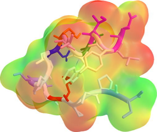
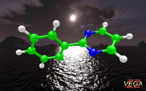
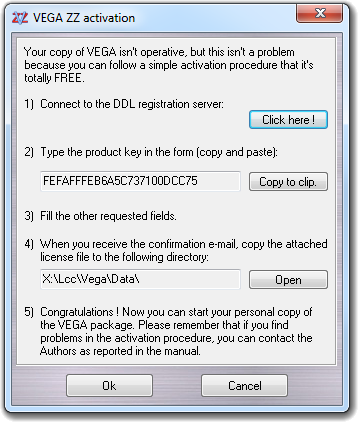
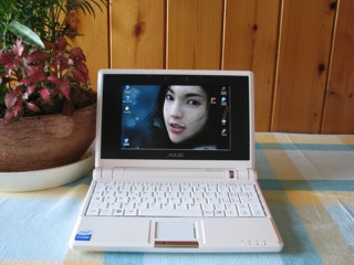
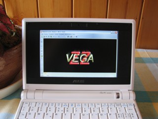
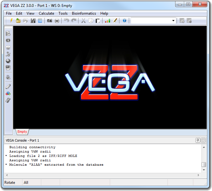
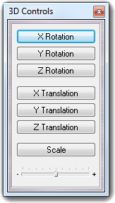
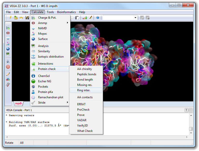
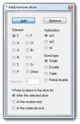
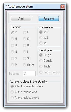
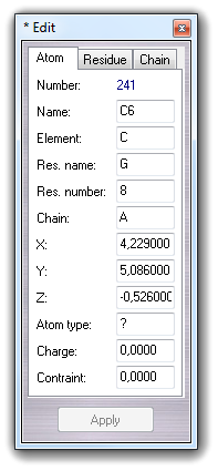
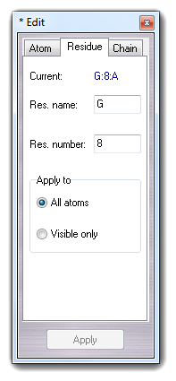
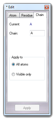
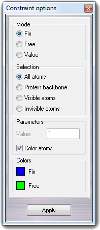
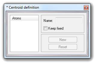
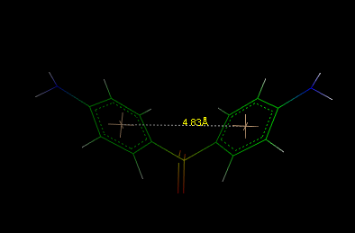
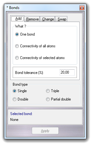
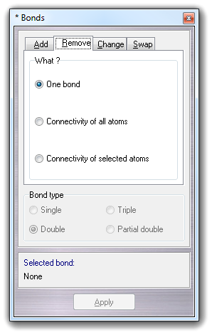
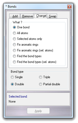
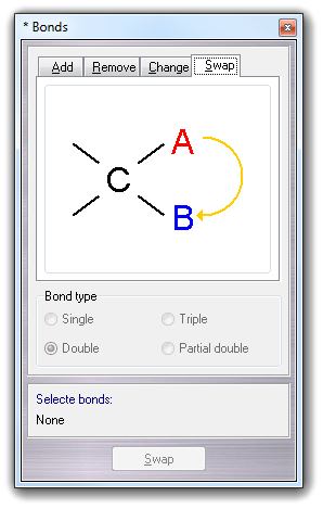
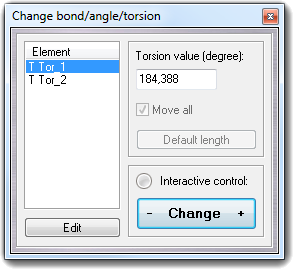
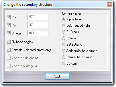
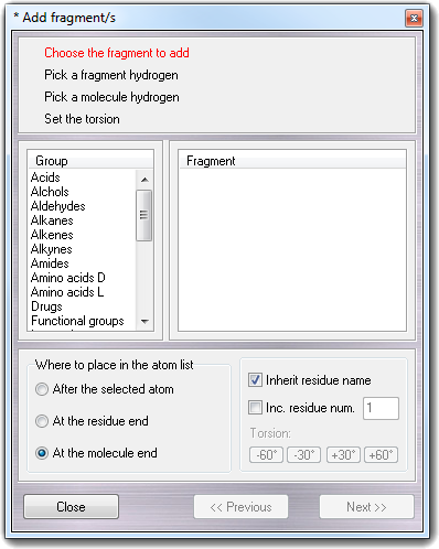
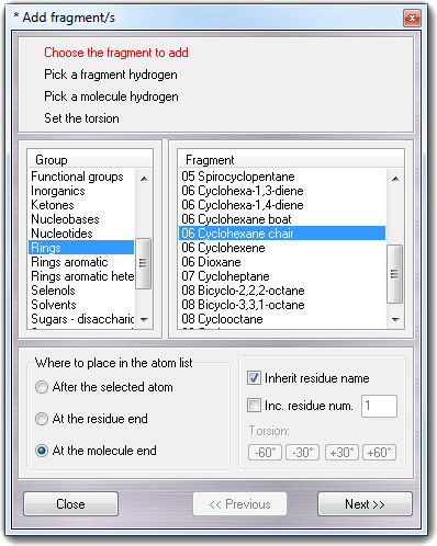
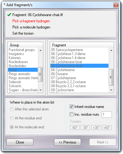
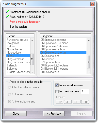
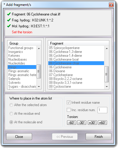
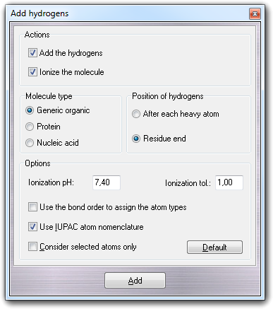
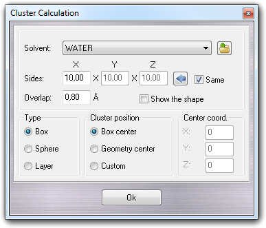
 button. The shape type (Box, Sphere and Layer)
influences the meaning of Sides fields. If Type is Box,
you can put the solvent box dimensions in Ångström. If Same is checked,
the box will be cubic. If Type is Sphere, you can put the Radius
of the cluster sphere in Ångström. If Type is Layer, you
can specify the thickness of the solvent in Ångström. Overlap
parameter indicates the maximum overlapping of the solvent-solute Van der Waals
spheres. In Cluster position you can choose where the cluster is placed
at the center of the box including the solute (Box center) or at the
barycentre of the solute (Geometry center ). When you select Custom,
you can specify the coordinates of the cluster centre. This feature is
useful when you have to solvate with an asymmetric cluster (e.g. phospholipidic bilayer)
and you want to place the solute in the middle. Checking Show the shape,
a preview of the solvent shape is shown making easier the cluster setup.
Clicking
button. The shape type (Box, Sphere and Layer)
influences the meaning of Sides fields. If Type is Box,
you can put the solvent box dimensions in Ångström. If Same is checked,
the box will be cubic. If Type is Sphere, you can put the Radius
of the cluster sphere in Ångström. If Type is Layer, you
can specify the thickness of the solvent in Ångström. Overlap
parameter indicates the maximum overlapping of the solvent-solute Van der Waals
spheres. In Cluster position you can choose where the cluster is placed
at the center of the box including the solute (Box center) or at the
barycentre of the solute (Geometry center ). When you select Custom,
you can specify the coordinates of the cluster centre. This feature is
useful when you have to solvate with an asymmetric cluster (e.g. phospholipidic bilayer)
and you want to place the solute in the middle. Checking Show the shape,
a preview of the solvent shape is shown making easier the cluster setup.
Clicking
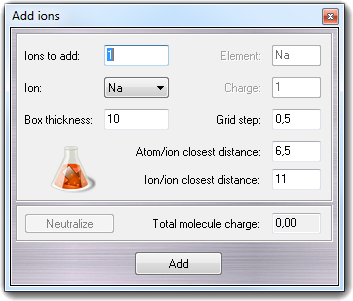
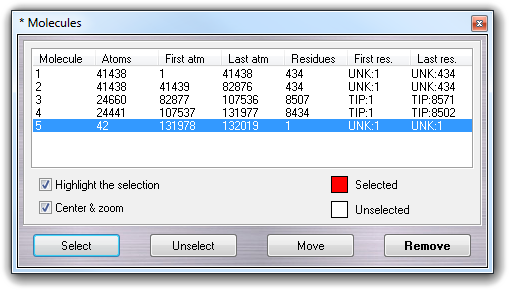
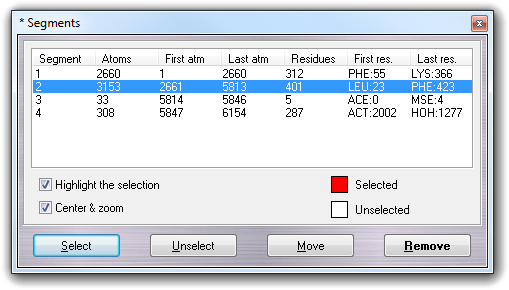
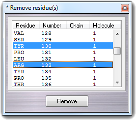
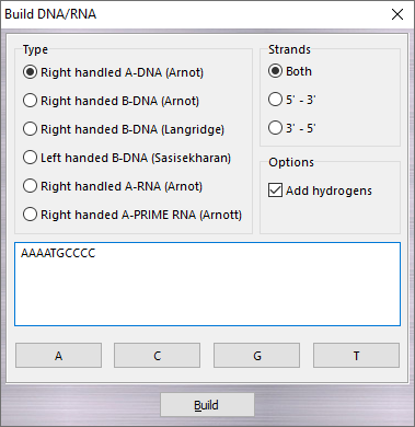
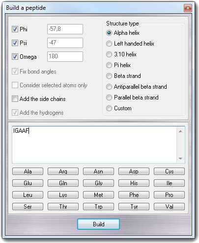
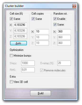
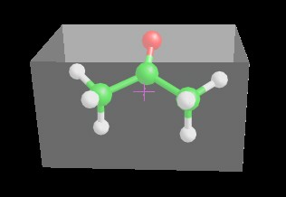
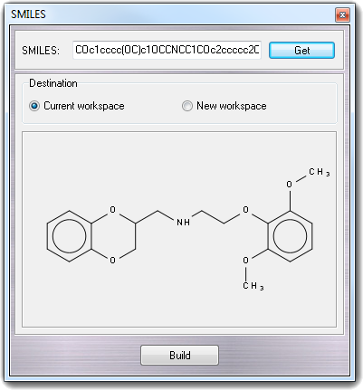
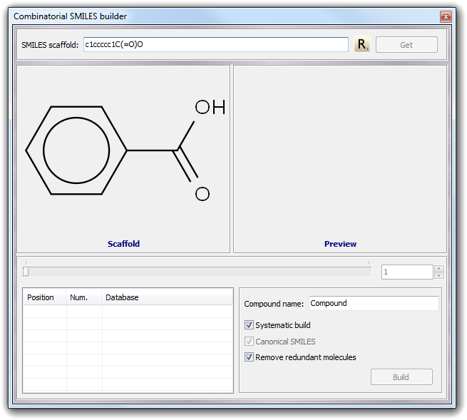
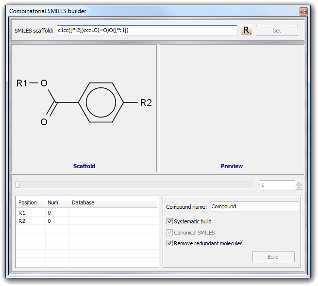
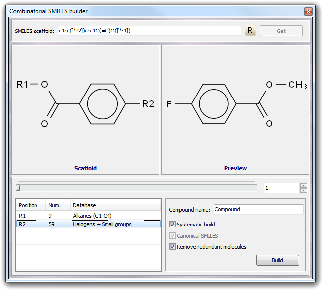
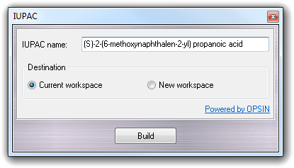
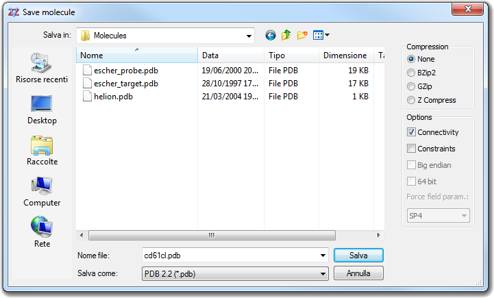
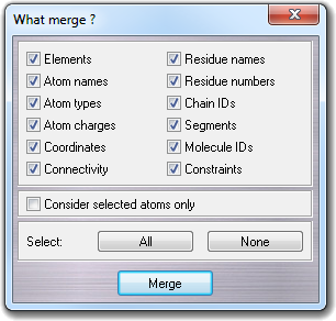
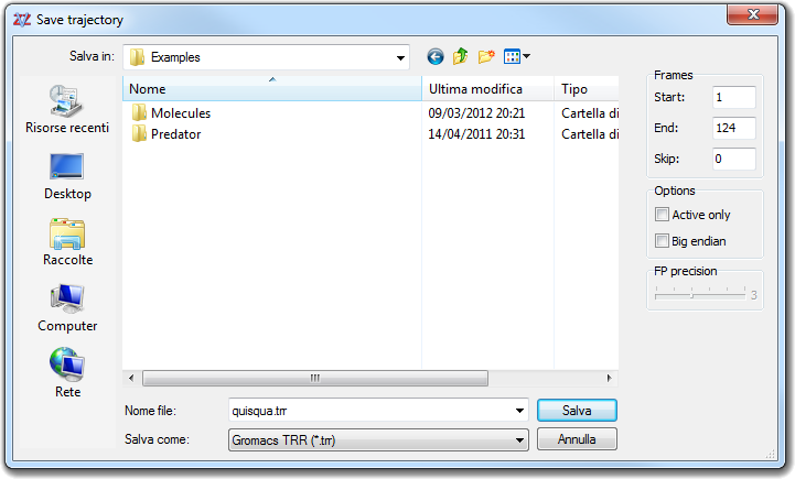
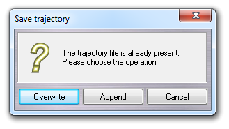
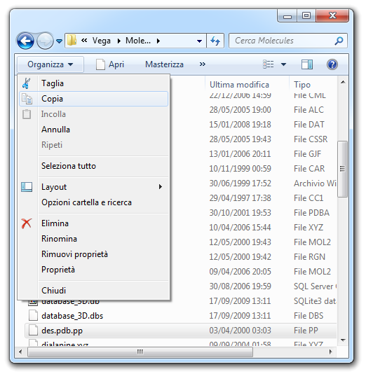
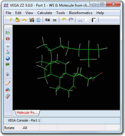
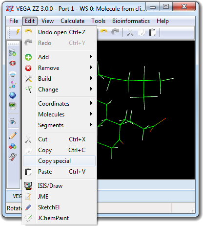
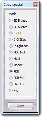
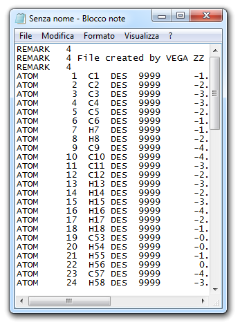
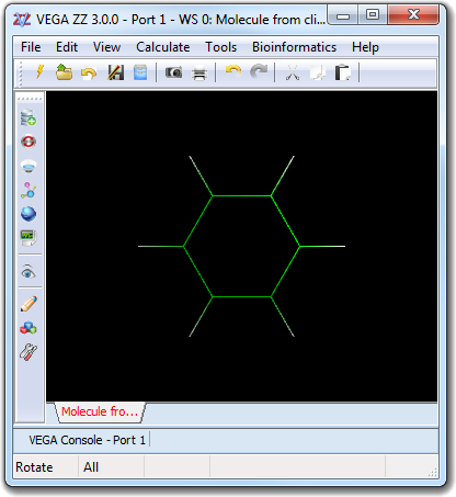
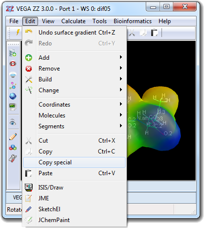
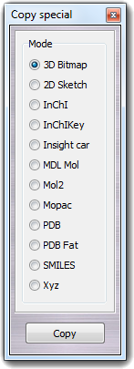
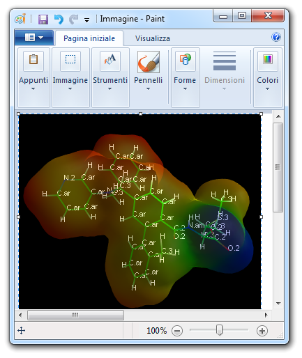
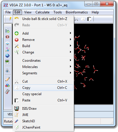
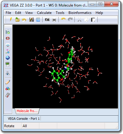
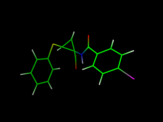
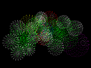
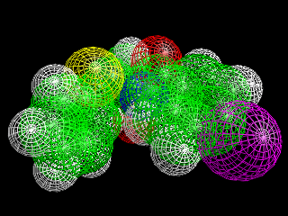
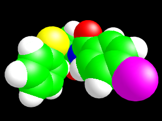

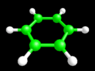
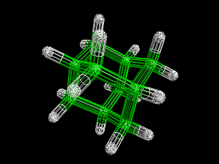
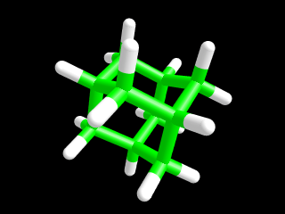
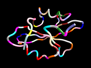
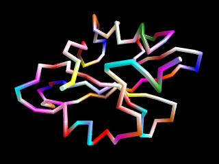
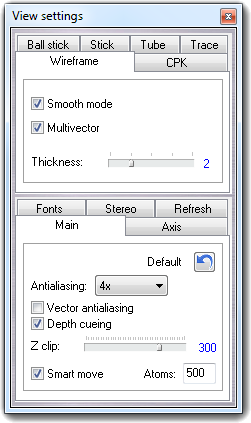
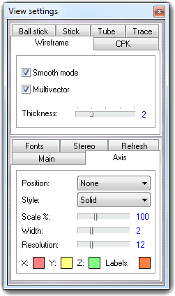
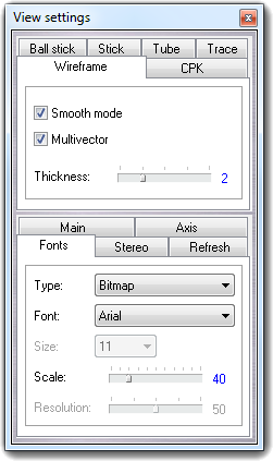
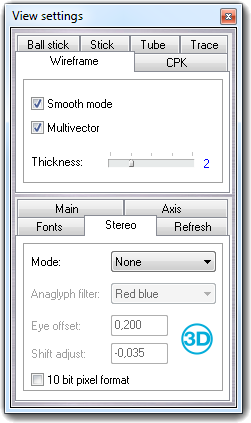
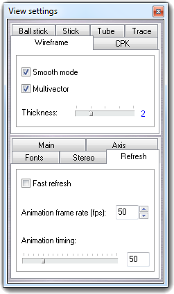
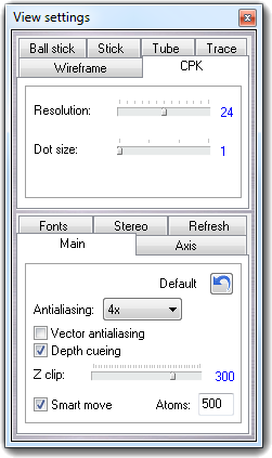
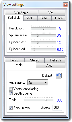
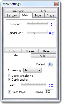
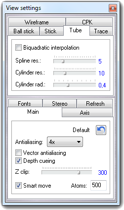
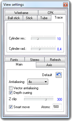
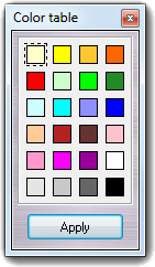
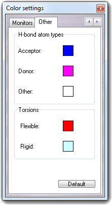 In
this tab, you can change the color of the H-bond acceptors, H-bond donors
and non H-bond involved atoms. Moreover, you can change the color of
flexible and rigid bonds.
In
this tab, you can change the color of the H-bond acceptors, H-bond donors
and non H-bond involved atoms. Moreover, you can change the color of
flexible and rigid bonds.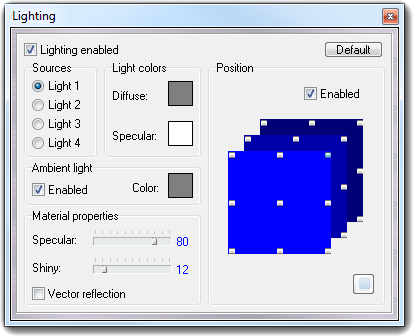
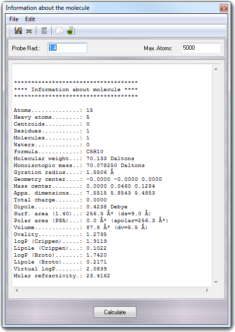
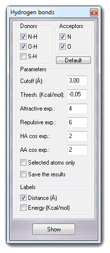
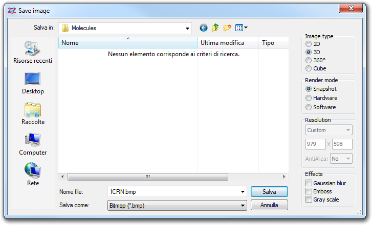


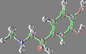
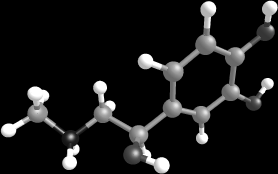

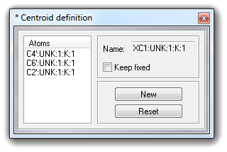
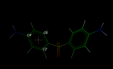
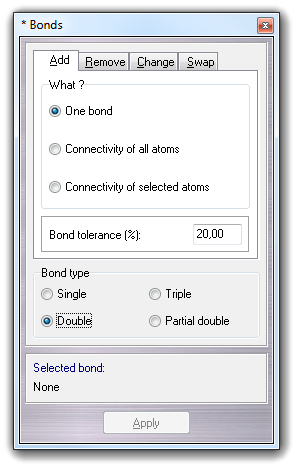

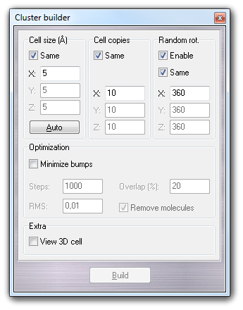
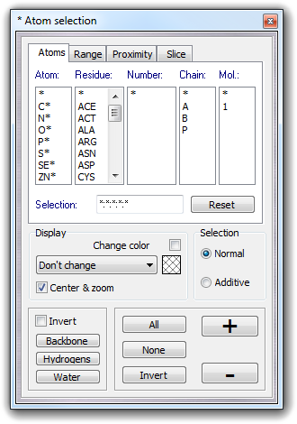 When the Atoms
tab is selected, it's possible show (
When the Atoms
tab is selected, it's possible show ( button) or hide (
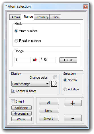 This operating mode is useful to select more than one atom in
sequence. You can specify the starting and the ending atom/residue number,
completing the Range
fields or clicking the structure in the main window. The
This operating mode is useful to select more than one atom in
sequence. You can specify the starting and the ending atom/residue number,
completing the Range
fields or clicking the structure in the main window. The
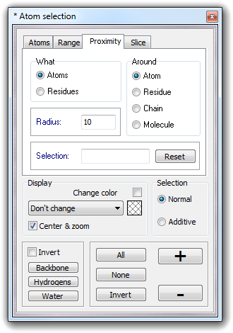 This selection mode is useful to un/select the atoms or
residues (see What box) around an atom, residue, chain and molecule
(see Around box). You must
specify the radius (see Radius field) of the sphere/spheroid and its
object center in the Selection field. Using the
This selection mode is useful to un/select the atoms or
residues (see What box) around an atom, residue, chain and molecule
(see Around box). You must
specify the radius (see Radius field) of the sphere/spheroid and its
object center in the Selection field. Using the
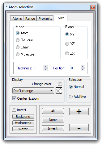 With
the Slice tab, you can un/select atoms, residues, chains and
molecules inside a user-defined slice: you can specify the
selection Mode (Atom, Residue, Chain and Molecule), the cut Plane
(XY, YZ, ZX), the slice Thickness in Å and the slice Position.
The
With
the Slice tab, you can un/select atoms, residues, chains and
molecules inside a user-defined slice: you can specify the
selection Mode (Atom, Residue, Chain and Molecule), the cut Plane
(XY, YZ, ZX), the slice Thickness in Å and the slice Position.
The


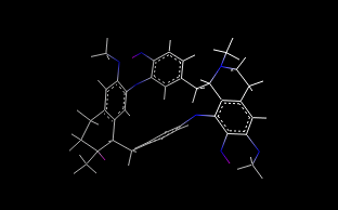
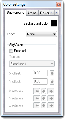
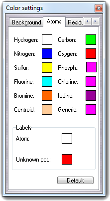 In
this tab, you can change the color scheme used when you select View
In
this tab, you can change the color scheme used when you select View
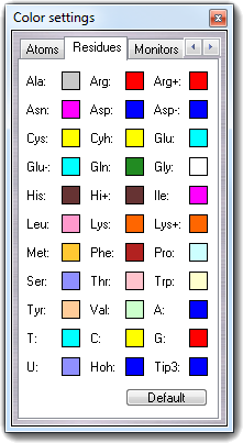 In
Residues tab, you can change the color scheme used when you select
View
In
Residues tab, you can change the color scheme used when you select
View
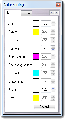 In
Monitor tab, you can set the color and the transparency (0 = full
transparent, 255 = full opaque) of the monitors shown when you measure
angles, bumps, distances, torsions and angles between two planes.
Clicking Default,
the colors and the transparencies are reverted to default.
In
Monitor tab, you can set the color and the transparency (0 = full
transparent, 255 = full opaque) of the monitors shown when you measure
angles, bumps, distances, torsions and angles between two planes.
Clicking Default,
the colors and the transparencies are reverted to default.